The Simulation of US Consumer Credit Fluctuation Using Artificial Neural Networks

Introduction

Following another paper that the researchers considered which can offer the groundwork for future research (see 16th IBIMA Conference), the authors try to find new techniques that can offer quicker and easier decision making tools.

The present paper takes into account one of the reasons for the 2008 financial crisis: the consumer credit. Furthermore, the researchers consider the US Consumer credit more importantly as it is one of certain considerations for the global economy evolution. The forecast of consumer credit, that the ANN can make, can be of paramount importance in a more and more volatile financial market and can be effective for quick decision thinking.

In order to simulate the CONS evolution, the researchers consider four indicators for the training of the ANN: Bank prime loan rate (LOAN), US Consumer Price Index Data (PRICE), Hires: Total nonfarm (HIRE) and US Total New Privately Owned Housing Units Started (OWN). The researchers believe that these four indices were sufficient for the training of the ANN, and also the researchers didn’t want to increase the number of inputs causing a huge amount of data. Moreover, the researchers thought that too many input indices represent too many data that the researchers must monitor in order to see how they influence the CONS. On the other hand, the researchers must not offer to the ANN a linear connection between input and output data.

The data used for the all the trainings and simulations were taken from Economagic.com website: http://www.economagic.com/ in September 2011. The data represent the monthly values of each of the input and output data from December 2000 until July 2011.

The objectives of the research are as follows:

1. Building, training and validating a specific ANN for the simulating of the Consumer credit outstanding (CONS), considering other four input data: Bank prime loan rate (LOAN), US Consumer Price Index Data (PRICE), Hires: Total nonfarm (HIRE) and US Total New Privately Owned Housing Units Started (OWN) in specific conditions;

1. Testing the trained ANN in order to check that the difference between the real data and the simulated to be smaller than 1.5%; 

1. Simulating the trend of CONS with the trained ANN;

1. Establishing the sustainability of future ANN use for the forecast of the CONS.

 
Artificial Neural Network (ANN)

Today Artificial Neural Network (ANN) can be found in the majority of human life activity, their potential being considered immense. The ANN are used in fields such as: data security, building security, medicine and pharmaceutics, research, meteorology, viniculture, finance and banks, social, space shuttle control, welding quality, automation, transport itinerary and human flux, speech, handwriting and face recognizing, manufacture etc. In the majority of these fields the ANN has as the main objective the optimizing of the processes and systems implemented into it. Starting with the human brain and continuing with the actual common application of the ANN, their use effectiveness is demonstrated as can be seen in Akira Hirose’s book “Complex-valued neural networks: theories and applications” [World Science Publishing Co Pte. Ltd, Singapore, 2003].

Regardless of the type, ANN has a few certain common unchallengeable elements, mentioned by Zenon WASZCZYSZYN in his book: “Fundamentals of Artificial Neuronal Networks” [Institute of Computer Methods in Civil Engineering, 2000]:

• Micro-structural components: processing elements – neurons or nodes

• Input connections of the processing elements 

•  Output connections of the processing elements 

• The processing elements can have optional local memory

•  Transfer (activation) function, which characterizes the processing elements.

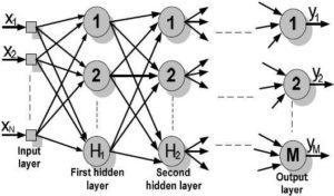
Figure 1. The Schematic Representation of a Multilayer ANN 

The schematic graphic representation of a multilayer ANN is presented in figure 1, were x_i ( ) is the input ANN values,  H1 and H2 are the numbers of neurons from the first and second hidden layer, M is the number of neurons from the output ANN layer and y_j ( ) is the values of the output data.

The Consumer Credit Outstanding (CONS)

The data which values are used are defined as following:

Consumer credit is (in millions of US$): “debt assumed by consumers for purposes other than home mortgages. Interest on consumer loans had been 100% deductible until the tax reform act of 1986 mandated that the deduction be phased out by 1991. Consumers can borrow through credit cards, lines of credit, loans against insurance policies, and many other methods. The Federal Reserve Board releases the amount of outstanding consumer credit on a monthly basis”. Definition is presented at http://www.allbusiness.com/glossaries/consumer-credit/4949780-1.html#ixzz1XSNnzM1U.

The researchers henceforward use the abbreviation CONS for this data.

For the simulation of the CONS, four input data are presented as follows:

Bank Prime Loan Rate (in %) can be explained as such: “The interest rate that commercial banks charge their most credit-worthy customers. Generally a bank’s best customers consist of large corporations. The prime interest rate, or prime lending rate, is largely determined by the federal funds rate, which is the overnight rate which banks lend to one another. The prime rate is also important for retail customers, as the prime rate directly affects the lending rates which are available for mortgage, small business and personal loans” at http://www.investopedia.com/terms/p/primerate.asp#axzz1XXQYybg9. The input values were found at http://www.economagic.com/em-cgi/data.exe/fedbog/prime and were renamed from now on as LOAN.

US Consumer Price Index Data (in %, when 1967=100) as is defined by the Financial Time lexicon: “The prices of consumer goods. These are normally measured by using a consumer price index, which shows the change over time in the price of a fixed basket of goods and services that would be bought by a typical consumer. This is the main measure of inflation in the economy” at website: http://lexicon.ft.com/Term?term=consumer-prices. The above price index has the starting calculation: 1967=100. The values used were renamed as PRICE and were found at http://www.economagic.com/em-cgi/data.exe/blscu/CUUR0000AA0.

Hires: Total nonfarm represents the number of total nonfarm US employees (x1000). Although nonfarm payrolls represent a very large portion of the US workforce, certain employees are not included in the nonfarm payrolls. Farm employees, self-employed individuals, employees on strike, employees on leave or laid off (even for a short period of time) are not included in the nonfarm payrolls total [http://www.investorglossary.com/nonfarm-payrolls.htm]. The researchers could find those data at http://www.economagic.com/em-cgi/data.exe/blsjt/JTS00000000HIL. The researchers also renamed them as HIRE.

US Total New Privately Owned Housing, as Units Started (x1000), is the number of new started to build houses, renamed for simplicity as OWN and its values are found at http://www.economagic.com/em-cgi/data.exe/cenc25/startssa01.

The researchers knew that the ANN can learn from the past CONS values, considering the four others inputs that the researchers decide to use, and they thought that the ANN will forecast accurate values of the CONS.

The values used for the simulation were taken from Economagic.com, Economic Time Series Page [http://www.economagic.com/].

Simulating the CONS Using ANN

Regardless of the ANN used, the processed data or the simulated problem, the phases in the implementation of ANN are the same, as shown by the authors in their articles. [Ilie C., Ilie M., Moldova Republic’s Gross Domestic Product Prevision Using Artificial Neural Network Techniques, OVIDIUS University Annals, Economic Sciences Series, Volume X, Issue 1, Year 2010, OVISIUS University Press, p. 667-672, ISSN 1582-9383]. Considering this, the following simulation follows those phases.

Phase 1 – Initial Data Analysis

Data analysis consists in dividing data into separate columns, defining types of these columns, filling out missing number values, defining the number of categories for categorical columns, etc.

Data analysis has revealed the following results:

• 5 columns and 119 rows were analyzed;

•  Data partition method: random

• Data partition results: 103 records to Training set (86.55%); 11 records to Validation set (9.24%) and 11 records to Test set (4.2%).

As the software is initially set to a partition of training: validation test is normally 60%:20%:20%, the difference shown above as 86.55%:9.24%:4.2% is a result of the researchers’ option. Considering the past experiences, the researchers wanted to determine a better training through a better number of training records (86.55% means 103 records) than 60% (71 records) of total records, even that the risk of ANN overfitting existed.

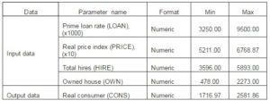
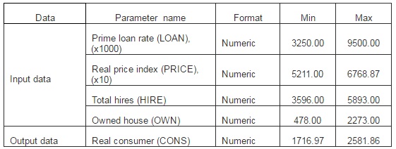
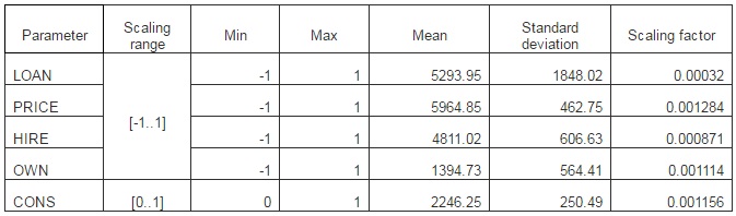
As can be seen, the database is divided in three sets. While the training sets are used only for training, the validation and testing sets are used also for testing. Presented in table 1 are the maximal and minimal value limits of the input and output data.

Table 1: The Database
 

Phase 2 – Data Pre-processing

This is the phase in which the above defined data are prepared and reshaped for an easier use and for obtaining best results, according to the requirements and the imposed results.

Pre-processing means the modification of the data before it is fed to a neural network. Pre-processing transforms the data to make it suitable for neural network (for example, scaling and encoding categories into numeric values or binary) and improves the data quality (for example, filtering outliers and approximating missing values), as different software uses different methods [De Xiaohui Liu, Paul R. Cohen,Paul Cohen, Advances in Intelligent Data Analysis1997].

Considering the past research and experiences, the database is reorganized as random series, replacing the initial time series. The reasons for this change came from the need to avoid the obstruction of the training and also the probability of the ANN to consider the trend of the time series database as universal trend. The second problem can be determined by the impossibility for future estimates. Also, the data values were modified in order to have the same level of admeasurement. For example, 521.1 original values from PRICE data became 5211 and 1716969.72 original values from CONS data became 1716.969.

So the data on which the ANN is trained were fed to it as non-time series, and for the present database the encoding chosen is numeric encoding. Numeric encoding means that a column with N distinct categories (values) is encoded into one numeric column, with one integer value assigned for each category. For example, for the Capacity column with values “Low”, “Medium” and “High”, “Low” will be represented as {1}, Medium as {2} and High as {3} [http://www.alyuda.com]. In table 2, the characteristics of pre-processed data are shown.

The results of completed pre-processing process are:

• Columns before preprocessing: 5;

• Columns after preprocessing: 5; 

•  Input columns scaling range: [-1..1];

•  Output column(s) scaling range: [0..1];

• Numeric columns scaling parameters: LOAN: 0.00032; PRICE: 0.001284; HIRE: 0.000871; OWN: 0.001114; CONS: 0.001156.

Table 2: The Pre-processed Database
 

Phase 3 – Artificial Neural Network Structure

Considering the characteristics of the simulated process, many ANN structures can be determined and compared through the specificity of the process and the data that are being used for simulations. Thus, the feed forward artificial neural network is considered the best choice for present simulation [Lucica Barbeş et all, Revista de chimie, Martie 2009].

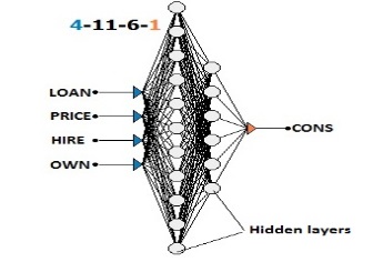
After building and testing several ANNs with feed forward structures, having in mind the comparison of the errors between the real data and ANN output data, the best ANN network is defined. This has the following structure (figure 2): 4 neurons in the input layer, 17 neurons in two hidden layer (first hidden layer – 11 neurons, second hidden layer – 6 neurons) and 1 neuron in output layer. This ANN structure is the result of several basic training having the goal to determine the fittest ANN for the database that the researchers used.

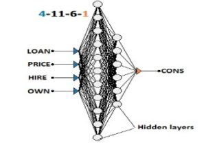
Figure 2. Simplified Graphic Representation of ANN with Structure 4-11-6-1

Even that it has been stated that in function approximation problems, the hidden layer activation function should be sigmoid-based, and the output layer activation function should be linear-based (the simplest activation function). The researchers have chosen for the hidden layers the hyperbolic tangent as the activation function (ratio between the hyperbolic sine and the cosine functions (or expanded, as the ratio of the half-difference and half-sum of two exponential functions in the points z and –z). This choice is considered because the researchers found, through experiments, that the hyperbolic tangent activation function offers a practical advantages of faster convergence during training and that should give a more close value of the training error [Irwin King, ICONIP 2006, October 2006]. The output layer activation function is a logistic function (sigmoid curve) [Dumitru Iulian Năstac, Reţele Neuronale Artificiale. Bucharest, 2000]. The researchers consider that the logistic function minimized the effects of overfitting that happened with the previous trainings when is used the linear function.

Phase 4 – Training

Being an essential phase in the use of ANN, the training must use certain training algorithms which essentially modify the structural elements of ANN (weights) through several iterations. Those modifications establish the future ANN accuracy. For the selected ANN, the most common training algorithm is Back propagation algorithm.

Back propagation algorithm: Back propagation is the best-known training algorithm for multi-layer neural networks. It defines rules of propagating the network error back from network output to network input units and adjusting network weights along with this back propagation. It requires lower memory resources than most learning algorithms and usually gets an acceptable result, although it can be too slow to reach the error minimum and sometimes does not find the best solution [Anupam Shukla, Ritu Tiwari and Rahul Kala, Towards Hybrid and Adaptive Computing, 2010]. For a quicker training process, a modification of the back propagation algorithm, called quick propagation, is made. 

Quick propagation is a heuristic modification of the back propagation algorithm invented by Scott Fahlman. This training algorithm treats the weights as if they were quasi-independent and attempts to use a simple quadratic model to approximate the error surface. In spite of the fact that the algorithm does not have theoretical foundation, it is proved to be much faster than standard back-propagation for many problems. Sometimes the quick propagation algorithm may be instable and inclined to block in local minima. [Fahlman, S. E., Faster-Learning Variations on Back-Propagation, 1988].

The training conditions were established in order to achieve the best results using the quick propagation training algorithm. Thus, the quick propagation coefficient (used to control magnitude of weights increase) is 0.9 and the learning rate (affects the changing of weights – bigger learning rates cause bigger weight changes during each iteration) is 0.6. The small values of these two, especially of the learning rate, are explained by the necessity of avoiding the local minima blockage.

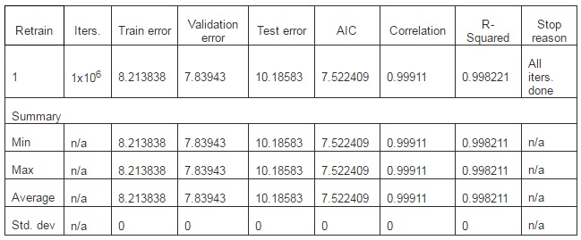
The stop training conditions were: maximum of 1000001 iterations or a maximum absolute training error equal with the value 1 tracked only on training set. The results of training are Number of iterations: 1000001 (Time passed: 00:34:06 min.). The training stop reason is: All iterations were done. After all iterations were done, the absolute training error is 2.605067. The systems configuration used to achieve that time is: Processor – Intel Core i3 CPU M330@ 2.13 GHz, Installed memory (RAM) – 3.00 GB and a 32-bit Operating System. The results of training details are presented in table 3.

Table 3: The Training Details
 

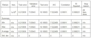
• AIC is Akaike Information criterion (AIC) used to compare different networks with different weights (hidden units). With AIC used as fitness criteria during architecture search, simple models are preferred to complex networks if the increased cost of the additional weights (hidden units) in the complex networks do not decrease the network error. So, the AIC should determine the optimal number of weights in neural network [Keith W. Hipel,A. Ian McLeod, 1994];

•  Iters. are the iterations [http://www.alyuda.com];

• R-squared is the statistical ratio that compares model forecasting accuracy with accuracy of the simplest model that just use mean of all target values as the forecast for all records. The closer this ratio is to 1, the better the model is. Small positive values near zero indicate poor model. Negative values indicate models that are worse than the simple mean-based model. Do not confuse R-squared with r-squared that is only a squared correlation [http://www.alyuda.com];

Training Results

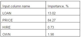
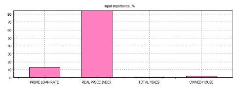
After the training, the ANN evaluated the importance that every input data has over the output data. The result of the evaluation is presented in table 4 and figure 3.

Table 4: Input Data over Output Data Importance

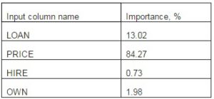
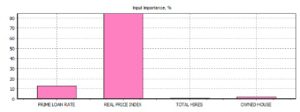
Figure 3. Input Data over Output Data Importance

In the next figures, the results of the training are shown as follows:

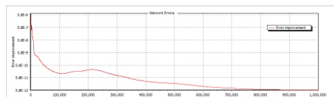
• Figure 4. Evolution of network error through the 1000001 iteration

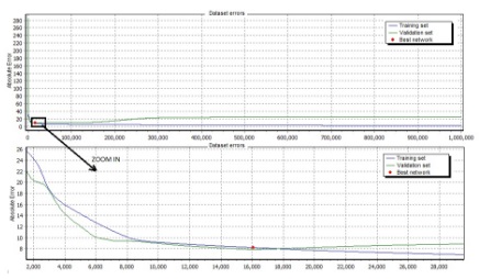
• Figure 5. Comparison between training set dataset errors and validation dataset error 

• Figure 6. Training errors distribution

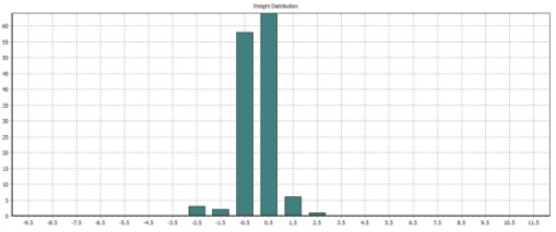
• Figure 7. Network weight distribution

Figure 4. Evolution of the Network Errors

 
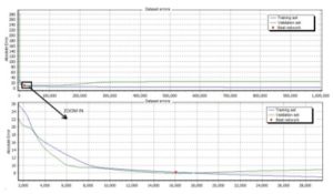
 Figure 5. Comparison between Training Set Dataset Errors and Validation Dataset Error

Figure 6. Training Errors Distribution

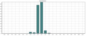
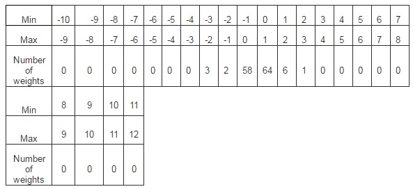
Figure 7. Network Weight Distribution

The weight distribution can also be seen in table 5.

Table 5. Number of Weights and Their Value Distribution

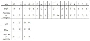
The number of iteration used (1000001) can give the impression that the ANN is overfitting. This is a risk that the researchers accepted and the result of ANN training, as the error value evolution (see figure 6), shows that the ANN is not overfitting.

 
Phase 5 – Validation and Testing

The last phases of ANN simulation indicate the level of ANN preparedness regarding the expected results.

Testing is a process of estimating quality of the trained neural network. During this process, a part of data that is not used during training is presented to the trained network case by case. Then forecasting error is measured in each case and is used as the estimation of network quality.

For the present research, two different sets of data were used for the testing and validation of the ANN training.

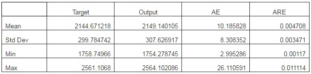
The first set is the one already used in the training process: 11 records to Test set (4.2%) (see phase 1), as a condition for training accuracy. The results of this testing is presented in table 6. Also, the difference between the real values (target) and the simulated values (output) of the output data are presented in figure 8.

Table 6: Test no. 1. Automat Testing Results – Actual Vs. Output
 

• AE is the absolute error as the difference between the ANN output and the actual target value for each data [Ajith Abraham, Bernard de Baets and all, 2006];

• ARE is the absolute relative error as the difference between the actual value of the target column and the corresponding network output, in terms of percentage [http://www.alyuda.com].

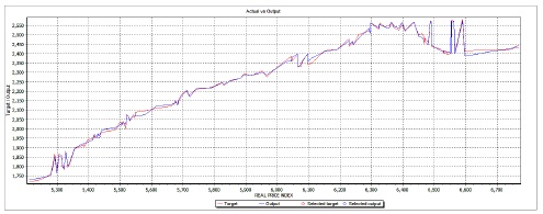
a) Actual Vs. Output Values. All Inputs

b) Actual Vs. Output Values. LOAN Values

c) Actual Vs. Output Values. PRICE Values

d) Actual Vs. Output Values. HIRE Values

e) Actual Vs. Output Values. OWN Values 

Figure 8. Actual Vs. Output Values. Automat Testing: a) All Inputs; b) LOAN; c) PRICE; d) HIRE; e) OWN

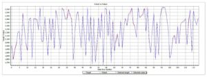
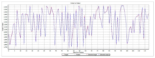
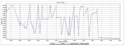
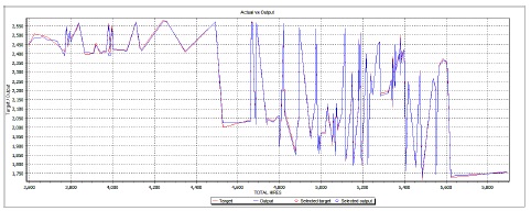
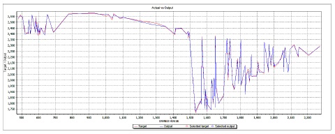
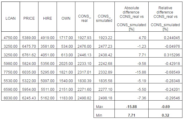
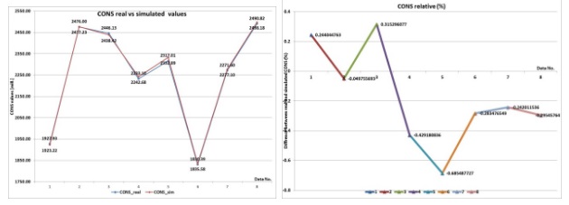
The second set is formed from data that were never feed to the ANN in order to train it. This second test set is chosen randomly from the entire database. The reason that the set doesn’t belong to a special cluster or period of time (like the period of time when the financial crisis start or act) is to see how the ANN answers any values, that even do not belong to the initial training data. So this set is new to the trained ANN. The results of the comparison between the real data and the simulated data are presented in table 7 and in figure 9.

Table 7: Testing Results – Actual Vs. Output
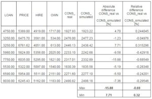
  Figure 9. Actual Vs. Outpt Values

From the previous results, the following conclusions are drawn:

•  The training phase is successful, the  maximum absolute error is 26.11059 and a maximum absolute relative error is 1.202656%;

• Testing the training with the new data set resulted in a smaller than 0.69% difference between the real data and simulated output.

Simulating the CONS Trend Using the ANN

The researchers have not only evaluated the success of ANN training by comparing the real input data with the ANN simulated data, but they have also observed the trend that ANN simulates considering new data for each of the inputs.

In order to see the way the ANN behaves after the training, the researchers fed the ANN with the new data, as consecutive values in arithmetic progression for each and every input, while the other four inputs remained the same as in training session. Then the researchers considered the trend of the new used data in comparison with the real trend. The researchers used the trend of the simulated data because, as the researchers expected, the simulated data were affected by the simulation errors and thus the trends will be easier to compare.

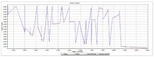
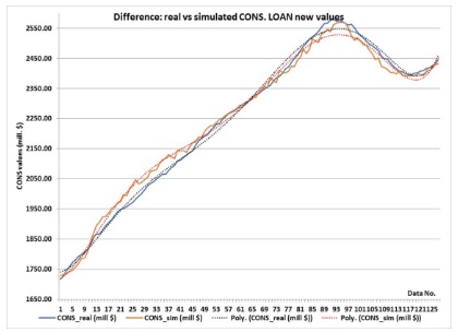
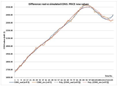
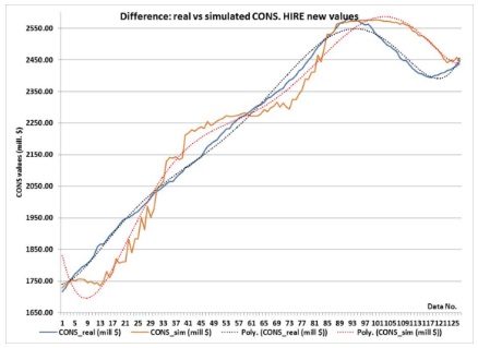
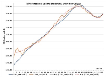
The researchers considered the results of CONS simulations for the new data (with consecutive values in arithmetic progression and all other inputs remaining as in original database). The trends graphic representations are shown in figure 10 for each of the input data. The two trends represented are in black – the trend for the real CONS values (Poly.(CONS_real)) and in red for the simulated CONS values (Poly.(CONS_sim)) in each of the next four graphics.

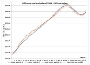a) Difference between Real CONS Values and Simulated Ones When the LOAN Values are Imposed

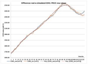b) Difference between Real CONS Values and Simulated Ones When the PRICE Values are Imposed

c) Difference between Real CONS Values and Simulated Ones When the HIRE Values are Imposed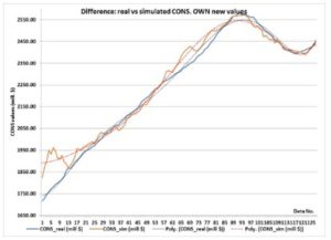d) Difference between Real CONS Values and Simulated Ones When the OWN Values are Imposed

Figure 10. The Comparison between Real CONS Values and Simulated Ones, When the INPUT Values are Imposed in New Consecutive Order

As can be seen, the ANN simulates the CONS’s trends with grate accuracy relatively to the real data. As expected, the more accurate ones are the trends of the LOAN and PRICE, as the trends of the HIRES and OWN contain a bigger amount of error.  This can be explained by the importance the ANN allocated for each of the input data (see Training results).

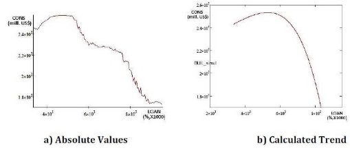
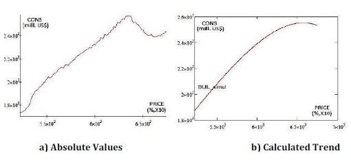
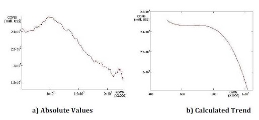
Next, the authors evaluate how the imposed data (for each of the inputs) determine the fluctuation of the CONS. After this evaluation, a calculation is made in order to determine the trend of the simulated CONS against each input, using the MATHCAD software. The results of these fluctuations and calculations are presented in the following four figures (from figure 11 to figure 14).

As can be seen in the above figures, the authors have determined the trends of the CONS for each of the input data. Further, the trends are used to show how CONS fluctuation when two input data are considered.

In figure 15, the 3D variation of the CONS simulated values is represented considering the determined trends of the each input data, based on the imposed data as consecutive values in arithmetic progression, for each and every input.

          
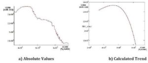
Figure 11. Simulated CONS Values When the LOAN Values are Imposed

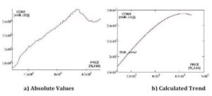
       Figure 12. Simulated CONS Values When the PRICE Values are Imposed

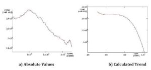       Figure 13. Simulated CONS Values When the HIRE Values are Imposed

 
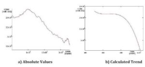
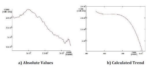
      Figure 14. Simulated CONS Values When the OWN Values are Imposed

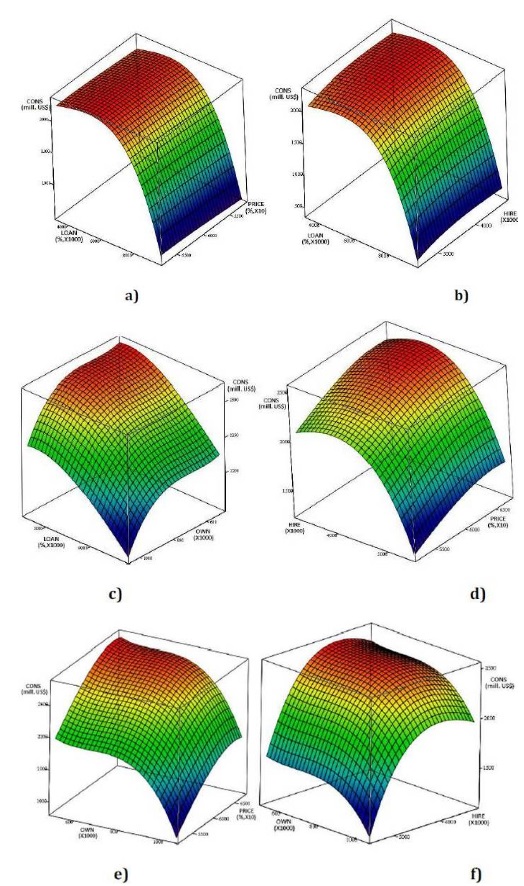
Figure 15. 3D Simulated CONS Variation When the Values are Imposed: a) LOAN and PRICE; b) LOAN and HIRE; c) LOAN and OWN; d) PRICE and HIRE; e) PRICE and OWN; f) HIRE and OWN.

Analyzing the 15^th figure, the following conclusion can be extracted:

• The LOAN has a stronger influence on the CONS then the PRICE and the HIRE as it can be seen in figure 15.a and 15.b;

• The LOAN has almost the same influence on the CONS then the OWN, but with a slight overcome, as it can be seen in figure 15.c;

• The HIRE has a stronger influence on the CONS then the PRICE, as it can be seen in figure 15.d;

• The OWN has almost the same influence on the CONS then the PRICE, as it can be seen in figure 15.e;

• The HIRE has a stronger influence on the CONS then the OWN, as it can be seen in figure 15.f.

Analyzing the above statements from the simulated data, it becomes obvious that the most influential data for the Consumer credit outstanding (CONS) is the Bank prime loan rate (LOAN) followed by the Hires: total nonfarm (HIRE) and US Total New Privately Owned Housing Units Started (OWN).

A small discussion must be initiated for the difference between the initial training importance of the input data (see training result – figure 5) and the simulated most influential data for the CONS trend. Even if the output data is the same, it must be considered that the ANN in the first case evaluates the numeric importance for the training accuracy. In the second case the influence is determined by the results of the training, as the ANN simulates the trends and shows which data is most influential for the trend evolution.

Acknowledgment and Conclusions

The research establishes the necessary theoretical characteristics for pre-processing, training, validating and testing the used ANN for the simulation of the US Consumer credit. Considering the validating and testing results, the ANN training is regarded as a success and all the initial conditions were respected.

In the beginning of the paper, the researchers show how the ANN is trained and tested. The results for the ANN training before the testing are:

• The training error is 2.50607;

• Network error 0.000026;

• The automat testing deviation of the training is [2.995286; 26.11] as absolute value and [0.00117; 0.011114] as relative value;

• The second testing (with data never feed to the ANN) results produced a relative deviation between [-0.69; 0.32];

All the tests confirm good results of the training process as the relative difference between the real CONS and the simulated CONS were smaller than the initial conditions (smaller then 1.5%).

Also the ANN training, validation and testing reveals that the most important factors for the Consumer Credit Fluctuation were the US Consumer Price Index Data and the Bank prime loan rate.

In the second part of the paper, the comparison between the real trends and the simulated trend proves the effectiveness of ANN building and training. The small difference between the two trends, even in harder conditions for the ANN, validates all the choices and restrictions that the researchers established for the ANN structure and training methods.

Also in the second part analyzing the CONS trend, the authors determine a hierarchy in what influences the Consumer credit outstanding. This hierarchy is different from the initial one that the ANN established in the training process (see figure 3). This difference emerges from the difference between the financial human behavior and the ANN training process.

Overall, the ANN training and use is considered a success and the future use of the ANN can be implemented for the forecasting of CONS for other countries and for financial and economical indices. But also the researchers consider that the studies must be extended over a larger period of time and over a bigger database. This can create a more prepared ANN, and thus a more accurate result. In addition, it is important to determine new indices that influence the consumer behavior in order to be used in ANN training.

References

Ajith Abraham, Bernard de Baets, Mario Köppen & Bertram Nickolay (2006). ‘Applied Soft Computing Techniques: The Challenge of Complexity  (Advances in Soft Computing),’ Springer-Verlag Berlin Heidelberg.
Publisher – Google Scholar 

Akira, H. (2003). ‘Complex-valued neural networks: theories and applications,‘ World Science Publishing Co Pte. Ltd, Singapore.
Publisher

Alyuda NeuroIntelligence – http://www.alyuda.com/neural-networks-software.htm

Anupam Shukla, Ritu Tiwari and Rahul Kala (2010).’ Towards Hybrid and Adaptive Computing: A Perspective,’ Studies in Computational Intelligence, Springer-Verlag Berlin Heidelberg, page 36.
Publisher – Google Scholar 

Barbeş, L., Neagu, C., Melnic, L., Ilie, C. & Velicu, M. (2009). “The Use of Artificial Neural Network (ANN) for Prediction of Some Airborne Pollutants Concentration in Urban Areas,” Revista de chimie, Martie, 60, nr. 3, Bucharest, p. 301-307, ISSN 0034-7752.
Publisher – Google Scholar 

De Xiaohui Liu, Paul R. Cohen & Paul Cohen (1997). ‘Advances in Intelligent Data Analysis, Reasoning about Data, Second International Symposium, IDA-97, London, UK, August, Proceedings,’ page 58.
Publisher – Google Scholar 

Dumitru, I. N. (2000). Reţele Neuronale Artificiale. Procesarea Avansată a Datelor (Artificial Neural Network. Advance Data Processing.). Printech Pub., Bucharest.

Fahlman, S. E. (1998). “Faster-Learning Variations on Back-Propagation: An Empirical Study,” Proceedings of Connectionist Models Summer School.
Publisher – Google Scholar 

Ilie, C. & Ilie M. (2010). “Moldova Republic’s Gross Domestic Product Prevision Using Artificial Neural Network Techniques,” OVIDIUS University Annals, Economic Sciences Series, Volume X, Issue 1, OVISIUS University Press, p. 667-672, ISSN 1582-9383.
Publisher – Google Scholar 

Ilie, C. & Ilie M. (2010). ‘Prevision Research of USA Retail and Food Services Sales Using Artificial Neural Network Techniques,’ OVIDIUS University Annals, Economic Sciences Series, Mechanical E  ngineering Series, Volume 12/no. 1, OVIDIUS University Press, Constanta, ISSN 1224-1776.

Irwin King. Neural Networks, Fuzzy Inference Systems and Adaptiv-Neeuro Fuzzy Inference Systems for Financial Decision Making, Neural information processing: 13th international conference, ICONIP 2006, Honk Kong, China, October 2006, Proceedings, Part III, page 434.

Keith, W. Hipel & McLeod, A. I. (1994). ‘Time Series Modelling of Water Resources and Environmental Systems,’ no 45, Elsevier Science B.V., page 210.
Publisher – Google Scholar – British Library Direct

Lucica Barbeş, Corneliu Neagu, Lucia Melnic, Constantin Ilie & Mirela Velicu. “The Use of Artificial Neural Network (ANN) for Prediction of Some Airborne Pollutants Concentration in Urban Areas,” Revista de chimie, Martie 2009, 60, nr. 3, Bucharest, p. 301-307, ISSN 0034-7752
Publisher – Google Scholar

WASZCZYSZYN Zenon (2000). ‘Fundamentals of Artificial Neuronal Networks,’ Institute of Computer Methods in Civil Engineering.

Xiaohui Liu, Paul R. Cohen & Paul Cohen. ‘Advances in Intelligent Data Analysis, Reasoning about Data,’ Second International Symposium, IDA-97, London, UK, August, 1997, Proceedings, page 58

Publisher – Google Scholar

http://www.economagic.com

http://lexicon.ft.com/Term?term=consumer-prices

http://www.investorglossary.com/nonfarm-payrolls.htm