Introduction
The need of new and cleaner sources of energy to replace conventional energies has been increasing over the years. Clean energy generation involves non-polluting sources or sources that have minimal negative effects on the environment, and is currently replacing a portion of the fossil-based power generation in many parts of the world. Among the clean energy technologies, wind energy power is one of the fastest growing in the global market, as Letcher (2008)points out in his book.The wind resource is a clean and renewable source found around the world for power generation, but it also represents a highly variable source of energy due to intermittency, climate variations, and other influential factors.
Along the years, different studies have been carried out to learn more about the behavior of the wind resource in order to determine the profitability and the performance of a projected wind power plant. Among these studies, it is worth to mention the work by Alawaji et al. (1996), who assessed the potential of the wind resources in Saudi Arabia. Alawaji et al., collected data from five monitoring stations and the wind direction, wind speed frequency distribution, mean wind speed and daily diurnal variation were calculated. Another example is presented by Zhou (2011) who assessed the wind resource in Juangsu, coastal province of China, with data from measuring stations and the help of aGeographic Information System (GIS) software for choosing possible places for installing wind turbines and determining array characteristics.
While the prices of oil and other conventional energies are on rise, the efforts to develop tools capable of predicting the wind resources and electrical production of a plant increase. The constant development and improvement of these tools allow the engineer to make more precise predictions and the reduction of uncertainty, which translates in better planning and utilization of wind resources.
In the investigation performed by Himria (2007), data from three measuring stations was employed to simulate a wind farm in each site using the RETScreen® software in order to carry out a prefeasibility study and obtain the appropriate conditions to install a wind power project. The work by Himria constitutes an example about how software could improve the wind resource assessment process.
In this paper, the prediction of electricity generation from wind resources using RETScreen® software (Clean Energy Project Analysis Software) is studied to determine the influence of different factors on the modeling of wind projects and to compare the energy production predicted by the software with the actual energy produced in operating wind farms. Establishing the influence of factors that affect the amount of electricity generated will ultimately permit to improve models and estimate the wind resource potential more accurately, and thus, accomplish a more reliable prediction of the economic outcome.
As summarized by the organization Cities Development Initiative for Asia (CDIA, 2011) pre-feasibility studies are carried out within a short time, in which different areas, such as the technical phases, the project development, risk analysis and financial feasibility must be covered if possible. In this stage the available data is often offered by local stations and public information, both of which are employed to model future projects with appropriate assumptions. After finishing this initial phase, a more detailed feasibility study is expected to follow it. The expected uncertainty level of a pre-feasibility study is approximately 20%, as compared with feasibility studies for which up to 10% differences are expected (CDIA, 2011). In wind energy generation projects, it is recommended to perform on site measurements at the selected place for the wind farm and to collect the necessary data for at least one or two years as it is mentioned by the Windustry (2014)and The New York State Energy Research and Development Authority (NYSERDA) (2010) .
RETScreen® isa free-to-use software based on MS-Excel, funded by the Canadian government, but it is not offered as an open source program; therefore, the user may select the parameters and their values, with possibility of programming add-on functionality, but without access to the source code.
The prediction of energy produced by wind farms is usually carried out through the estimation of power generation and potential losses. Several probabilistic and mathematical models have been developed to estimate the wind resource. These include different methods for calculating the Weibull distribution and shape factor, typically used to represent the wind resource frequency distribution in a given location as Pérez (2008) exposes in his work.
Among the aspects that influence the modeling of wind projects in RETScreen®, the Hellman exponent is one of the most relevant. The Hellman exponential law determines how the wind speed varies with respect to height and terrain roughness. Range of values for the Hellman exponent, named also ¨wind shear exponent¨, according to terrain type, are available in different sources, as for example in Díaz’ work(1993).
Previous statistical studies of the wind resource in nine wind farms located in Ontario, Canada, have been carried out to determine correlations between wind resources and operational parameters. The work of El-Mazariki (2011) has demonstrated the relevance of statistical methods to determine the influence of different factors on the modeling of wind energy (El-Mazariky, 2011). In the present work, twelve wind farms located also in Ontario, Canada were modeled using RETScreen® software and results were compared to actual measurements.
Wind Energy Production in Ontario
Currently, there is a large number of countries with a growing wind generation capacity. In fact, according to the Canadian Wind Energy Association (2013), Canada has a wind energy production of approximately 6.5GW, which supplies around 560, 000 homes and is equivalent to 3% of the total electricity production of the country. Data from the publication Power to Ontario (2013) suggests that the province of Ontario in Canada is one of the main producers of wind-based electricity in the country, with fifteen wind farms in operation and approximately 1.5 GWof installed capacity connected to the grid by 2012.
In-depth knowledge of available wind resources in a specific area is critical for corporate investors to determine if a project is profitable in that region. Wind speed is the most important factor in the prediction of energy production by a wind farm. However, there are other factors of considerable importance.
Twelve wind farms located in Ontario were modeled using RETScreen®. The results obtained are compared with experimental data from the aforementioned wind farms. The main objective of this study is two-folded in determining key parameters associated to the software prediction capability and thereafter, developing a complementary modeling criteria to enhance the use of it.
Influential Factors on Wind Assessment Prediction Using RETScreen®
In this section, the influence of the distance from meteorological station to wind farm, and topography when using RETScreen® software is studied in order to assess their effect on the predictive ability of the software.
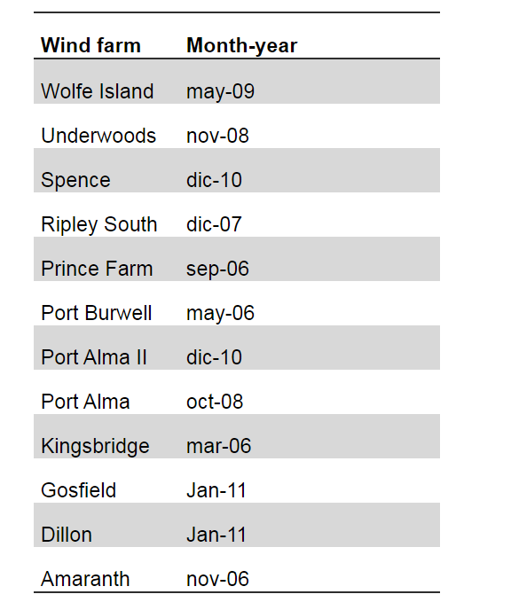
The energy production of 12 wind farms located in the region of Ontario was taken into consideration. Data available in the publication Power to Ontario (2013) starting on March 1st-2006, was used. Table 1 shows the starting date of operation for each wind farm considered.
Distance between Measuring Station and Production Site on Model Prediction
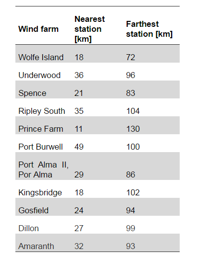
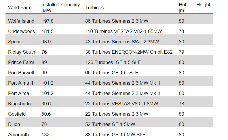
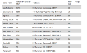
Three or four measuring stations for each wind farm were selected. The first station is the closest one to the given site, while the rest were chosen to cover a radius of approximately 130 km around the site. Table 2 presents the distance between each wind farm and its corresponding closest and farthest stations. The stations and the distances were selected from RETScreen® Plus version, which has direct access to NASA data of meteorological stations. For this study, only ground monitoring stations were selected. The average wind speed measurements correspond to a height of 10 meters above ground, standard parameter according to (EPA, 1987), and (WMO, 1983). Table 3 shows the number and type of turbines associated to each of the studied wind farms according to Ontario Power authority (2014).
Table 1: Start Date of Operation of Wind Power Plants in Ontario, Canada
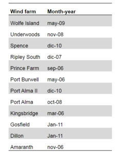
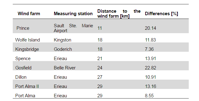
Table 2: Distance between Measuring Stations and Wind Farm
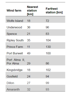
Table 3: Turbines in the 12 Wind Farms
Thereafter, the electricity production was modeled for each wind farm with the information provided by the selected meteorological stations surrounding it. These results were compared with the measured energy production. The quality of the prediction was studied as a function of the distance between the wind farm and each of the measuring stations associated to it. This study was carried out for all twelve selected wind farms.
Default values were chosen for the wind shear exponent (0.14) and shape factor (k=2) in the software. The software database provides a 10-year average wind velocity for each measuring station to be used in the calculations. In our model, we considered the following losses: array losses (1%), airfoil losses (1%) and miscellaneous losses (2%). The availability was considered as 98%.
Results include annual energy production for the model according to the studied wind farm, which will be called hereafter, predicted energy and will be compared with the measured production of the wind farm for a determined year (according to the starting date of operation of the plant).
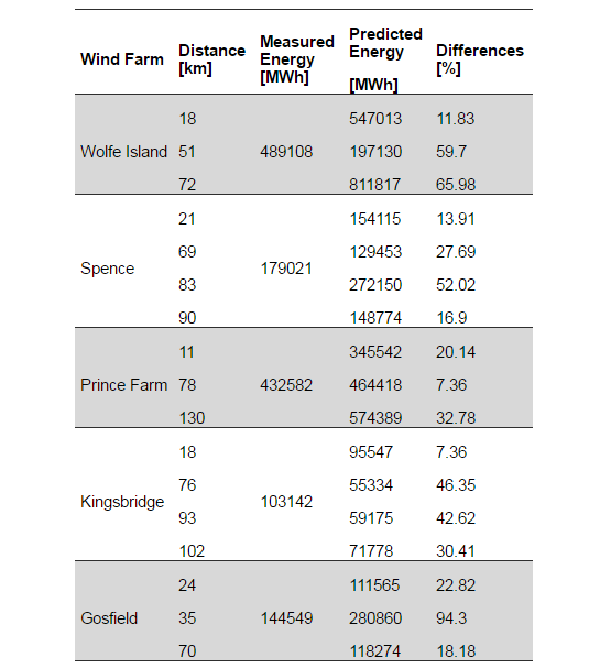
The results, as expected, show the smallest deviation between electricity predicted and measured production when the closest station to the wind farm is used. These results stand for nine of the twelve studied wind farms. In four of these nine wind farms (Wolfe Island, Underwood, Amaranth and Dillon) the quality of prediction decreases as distance between the measuring stations and the corresponding wind farm increases. This is not the case for the other five stations (Kingsbridge, Port Alma I, Port Alma II, Ripley South and Spence) of these nine wind farms, which show an erratic behavior farther from the closest station.
The other three wind farms (Gosfield, Port Burwell and Prince Farm) of the total twelve present the lowest differences between predictions and measurements for stations located farther from the wind farm than for the closest measuring station. This could be for two possible reasons;the first one is a high variability in the wind speed in the closest measuring station, which could affect the quality of the prediction when this data is employed. To test this hypothesis, the variability of the wind speed was quantified using the standard deviation for the closest measuring station of all twelve wind farms. However, a significant trend could not be identified. The second possibility would be that the measuring stations with lowest differences, which are farthest to the wind farm, just by chance, have a better match with climatologic conditions found in the wind farm, but not due to a real correlation. As shown in Table 4, the farther stations are at least 70km away from the wind farm and quality of the prediction could be erratic. This is supported by the fact that 9 out of 12 wind farms present high differences when the farthest wind farm is considered.For brevity, a representative sample of the obtained results is shown in Table 4 with five studied wind farms of the total twelve.
Table 5 shows the differences found between electricity productions and predicted for stations located at 30 km or less from eachof the 12 considered wind farms. The maximum difference is 23%, while the minimum is 7%. These errors give a reference about how far a measurement station could be located in order to perform a pre-feasibility study and the level of uncertainty associated with the distance.
Although several measuring stations with different characteristics were studied, some similarities and common trends between them were found, which suggests that the conclusions of this study could be extended to other stations. Nevertheless, it is recommended to increase the number of studied wind farms in a future work in order to decrease the uncertainty level. For this particular set of wind farms, results demonstrate acceptable differences when data from a weather station within 30 km to the wind farm is taken. If no measuring stations at less than 30km are available, it is recommended to pay special attention when selecting the closest station as this choice may lead to unacceptable uncertainties.From here on, the closest station to the wind farm was employed to model the wind farms in RETScreen® V.4.
Table 4: Differences between Measured and Predicted Production of Electricity according to Wind Farm-Station Distance
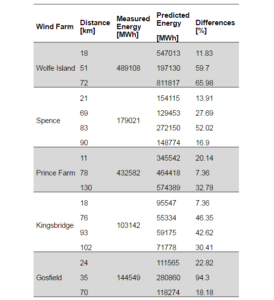
Table 5: Differences between Predicted and Measured Electricity Production in a Radius of 30 Km from the Wind Farm

Inluence of Topography on the Quality of Prediction
Since all 12 wind farms have different surrounding topographies, the next step was to include this variable to find out its influence in theseobserved levels of error. According to fundamentals of topography exposed in González (2012), the terrain surface may be classified as: plain, plateau, valley, foothill or mountain to describe the natural form, relief and landscape of a region.
To determine the influence of topography on the results, another study was addressed within a radius of 30 km of the wind farm. Nevertheless, despite the fact that all the wind farms and weather stations in this study have different topographies, the data available seemed insufficient to determine a correlation among electricity predicted production and only the distance and topography. Therefore, a more complete set of input variables was considered in the next sections.
Variations of Parameters in RETScreen ® v.4 Modeling
In this section, the variation of the prediction accuracy as a result of varying the shape factor, wind shear exponent and themethod of calculation of the average of velocityas input parameters was assessed. All twelve regions were considered in the analysis.
For this study, the average of the velocity was calculated by two methods. The first method employs Eq. (1) and data from NASA ground stations. In order to select meaningful, but uniform data among the different wind farms, a 5 years period was chosen for this calculation method, which corresponds to the statistic mode of the wind farms’ operation time. Equation 1 shows a proposal of average velocity according to Matthew (2006)who suggests that in the wind energy calculations, the average of velocity should be carried out according to its intervention in the power calculation. For this reason the average involving the velocity raised to the third power is used as one of the calculation methods:
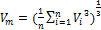 (1);
(1);
Where V is wind velocity and n is the number of hourly points read in a given station throughout the 5-year period.
The second method is the 10-year average velocity provided by the software with data from the same ground stations. Differences between the results from these methods are expected due to the quantity of years taken into account and the different expressions to calculate the average velocity. Both methods will be compared to determine which is more appropriate.
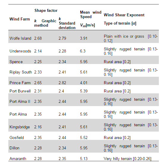
The shape factor permits to figure the distribution of wind speed along the year based on data for given period of time (5 years in this case) and its corresponding average velocity. This factor is obtained by two methods: the graphic method by Weibull distribution and the standard deviation method; both methods use the average velocity calculated through Eq. (1). These values were compared with the recommended-default value of the software, which is a shape factor = 2.
The type of terrain refers to the roughness of the terrain, i.e., the resistance to airflow due to the presence of obstacles, which modify the wind profile such as grass, buildings and trees. The roughness of the terrain is represented by the wind shear exponent and it is different to the topography, which is related to natural formations such as mountains and valleys in a region.
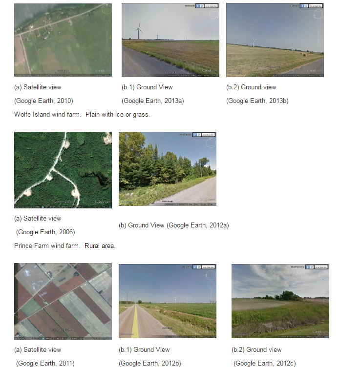
The free application Google Earth provides information about geographical coordinates, height above sea level of the studied wind farms location and pictures of the studied terrain. Once the wind farms are located in the application, the height above the sea level was studied in a radius of 40km and using images of each wind farm area, the type of terrain of the wind farm was visually determined.
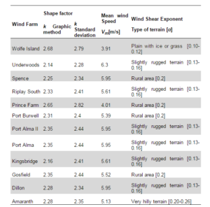
Finally, the wind shear exponent was chosen based on these observations and on the classification according to terrain type available in Díaz’ work (1993).Figure 1 shows an example of three wind farms and the type of terrain associated to each picture, and Table 6shows the selected parameters for each wind farm.
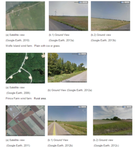 Port Alma y Port Alma II wind farms. Slightly rugged terrain
Figure 1: Wolf Island, Prince Farm, Port Alma and Port Alma II Satellite View and Ground View by Google Earth
Table 6: Matrix of Input k, Vm and α
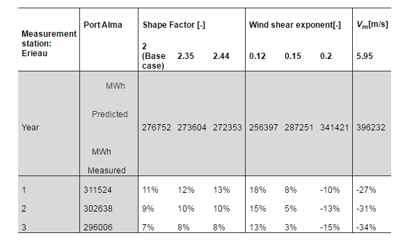
The modeling factors were evaluated as follows: firstly, the recommended values of the software were chosen; this condition is called base case. Afterwards, proposed cases were generated by modifying the base case, changing only one of the studied parameters at a time, while keeping the rest of the parameters at their default values. An example of the input variable settings in Port Alma wind farm is shown in table 7.
Table 7 shows the difference between the predicted energy obtained by the variation of the parameters, and the measured energy in the wind farm for three consecutive years (from the starting date of operation of the wind farm up to the latest available data). Thus, it is possible to observe how the variation of these parameters affects the quality of the prediction and if the observed results are independent of the selected year.
The differences between the measured and predicted electricity generation are represented in [%]. If the percentage is positive, it means that the production in the wind farm was higher than the predicted production and viceversa.
This process was carried out for the twelve wind farms and it was found that, for the shape factor input parameter, the best approximation is the base case k=2. Nevertheless, the differences between k taken in the base case and the values calculated by graphic and standard deviation methods were less than 5%.
For the calculation of the mean velocity, when (1) was employed, the differences increased more than 20% in comparison with the base case (average provided by the software). The latter is then recommended instead of the initially proposed expression. The software provides an average velocity with ten-year hourly measurements, allowing it a better understanding of the meteorological conditions in a specific location.
For the wind shear exponent, it was found that the results could certainly improve (about 3% in this case) according to the proper consideration of type of terrain. The next section contains a more detailed study about this factor and its influence on predictions.
According to the study, after varying the three selected parameters, the prediction of electricity generation in ten out of the twelve wind farms maintain the same trend: the results improve with the selection of an adequate wind shear exponent according to the type of terrain. However, for the other two parameters, shape factor and average wind velocity, the best results were found employing the values recommended-defaulted by the software (the base case).
Nonetheless, the remainder two wind farms, Amaranth and Port Burwell, had high differences respect to their respective measured energy. In Amaranth, for the base case, the predicted energy differs more than 50% from the measurements, while the proposed case was off by 20%, which means that predictions with the default parameters (base case) and those set in our proposed case were quite inaccurate for a prefeasibility study in this wind farm; this is a possible consequence of the very hilly type of terrain. Port Burwell wind farm was dismissed since the average wind speed (10 years average) in the closest measuring station is 2.7 m/s, which is lower than the wind turbine cut-in speed. This means that just a tiny fraction of time will be useful for electricity production according to the shape factor used, and hence, the energy predicted by the software would be almost null.
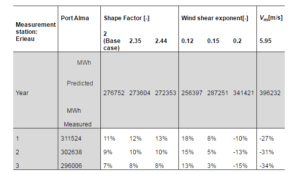
Table 7: Base Case and Parameters Variation for the Port Alma Wind Farm
Wind Shear Exponent Range Analysis
The proposed cases where the wind shear exponent was modified according to the observed type of terrain show smaller differences with the measured data than found in the base case.The proposed case using a wind shear exponent different to α=0,14 (default value) can improve the quality of the results in some cases. To assess this improvement, the following procedure was followed: after selecting the wind shear exponent range for each region, the energy production was predicted changing only this parameter and using the suitable values of wind shear exponent per region.
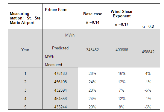
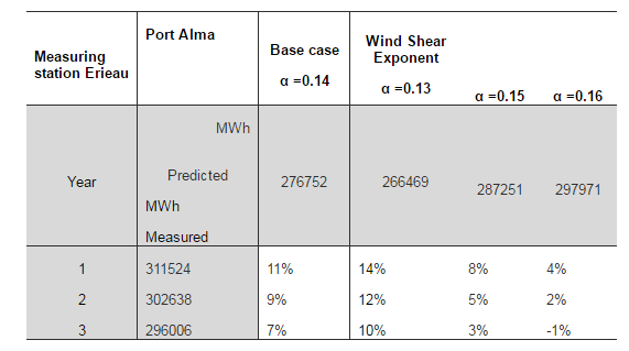
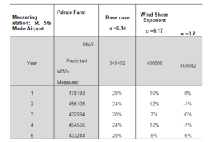
The results forall of the modeled regions were similar. Two regions with different types of terrain are shown in tables 7 and 8 (Prince Farm and Port Alma, respectively). In both tables, it is possible to observe the differences in the quality of prediction between the base and proposed cases, where the boundaries of the selected range of the wind shear exponent are evaluated. Results are shown for 5 consecutive years for Prince Farm and for three consecutive years for Port Alma in order to corroborate that the model provides similar quality of prediction, irrespective of the studied year.
Prince Farm (see Table 8) corresponds to a rural area, with a wind shear exponent ranging in the interval α=[0.17-0.20]. The base case was compared with the proposed cases and a reduction in the error of the results was found using the boundaries of the selected range. For the base case, the maximum difference found was 28% and the lowest was 20%, while for the boundaries of the range, differences were lower.For α=0.17 the maximum difference between predicted and measured electricity production was 16%, while for α=0.2 the maximum difference was 6%, even less than the minimum difference in base case
Table 8: Wind Shear Exponent Analysis for Prince Farm
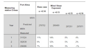
For a slightly rugged terrain, an example using Port Alma wind farm is shown in Table 9. The wind shear parameter ranges from α=0.13 to 0.16 (passing by 0.14, which corresponds to the base case). Using α=0.13 the difference between prediction and measurement shows a slight increase of 3 percentage points respect to the base case, whilst using α=0.16 it led to the lowest difference of 1percentage points. For α=0.15 the difference was 3 percentage points lower than for the base case.
After completing this study for all the regions, it was found that for slightly rugged terrain, it is possible to use α=0.15 as a default approximation instead α=0.14, which is the value used in the base case. The results improved at least 3 percentage points in the worst case scenario. This trend is the same for all six regions with this type of terrain. The results for rural areas show that it is possible to increase the quality of the predictions at least 4%, while for plain areas, such as Wolfe Island, an improvement of 9% was found when using α=[0.10-0.12], with respect to the base case. Selecting the correct value of α in a given region could reduce appreciably the difference between the measured and predicted electricity generation, especially in rural and plain areas.
Table 9: Wind Shear Exponent Analysis for Port Alma
Study of Variations of Meteorological Conditions
The variation in the prediction of electricity production was also scrutinized when actual weather conditions of one specific year, such as pressure, temperature, wind speed, and humidity are employed instead of selecting the 10-year average value suggested by the software by default. Only in this part of the study the predicted energy is calculated with data from one year of weather measurements. The predicted energy is compared with the actual energy production. This analysis is not reported in this paper, but is included in the thesis that supports this investigation (Romero Vergara, 2012). Considering that available data is from the nearest measuring station, which has a distance to the studied wind farm, it was demonstrated that climatic conditions measured during one specific year in a determined measuring station do not describe the climate of a specific region, while an average of 10 years does provide a better approximation of the typical conditions of an area where the wind farm is located.
Analysis of Variance for Non-Meteorological Factors
ANOVA (Analysis of Variance) was also employed to further determine the correlation between the topography and type of terrain with the electricity prediction by the software. In this part, we also added the brand name of the turbine as an extra parameter, since the software provides a handy set of brands and models with their manufacturer power curves.
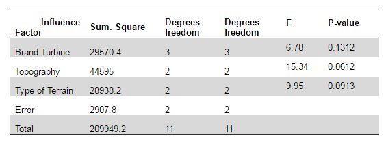
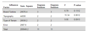
The null hypothesis is the position that there is no relationship between two measured phenomena. The objective of ANOVA is to evaluate the truthfulness of the null hypothesis through the study of the variance between groups, i.e., to determine if the observed phenomena or variables are related. In order to do so, two parameters are compared: the significance level and the P-value. As explained by Montgomery et al., (2007) the former is the probability of mistakenly rejecting the null hypothesis and typically a value of 0.05 is used. The latter is a parameter associated to each independent variable considered and it represents the variable’s smallest significance level.If the P-value is lower than 0.05 for a given variable, a 95% probability of it being correlated to the dependent variable exists.The smaller the P-value is, the more convincing the evidence is against the null hypothesis. In this case, the dependent variable is the daily electricity production per wind farm and the independent variables are the brand of the turbine, the topography and the type of terrain. The result of the ANOVA is shown in Table 10.
The study shows a P-value between 0.06-0.13 for all independent variables, which means that they do not have strong influence on the wind generation model. This is understandable because, it is not possible to define a model with these three parameters alone, although some of them have a P-value near 0.05. Results from ANOVA show the order of influence: first the topography, then the type of terrain and at last the brand of turbine. This means that the selection of these factors may contribute to the quality of the model, but their influence may be negligible on the prediction. Using a larger sample of wind farms is recommended for confirming this trend for other regions.
Table 10: ANOVA
The shape factor led to consistently better predictions of electricity generation when taken as k = 2 from the Rayleigh distribution. Use of alternative methods to determine k from the available wind data did not prove to be better than using the default value in these regions. The differences between these methods were around 5% in favor of using the default k.
In the evaluation of the wind speed, it was concluded that using the average measurement at the closest station calculated by the software offers better results than the average of the calculated cube of the speed. The software provides a 10 years average wind speed, which gives a better understanding of the weather condition of an area.
A precise selection of the wind shear exponent according to type of terrain may reduce disparities in at least 4 percentage points for rural areas and 9% for smooth terrains. For slightly rugged terrain, it was found that it is possible to use the recommended exponent (α = 0.14) to obtain an acceptable prediction. However, using a wind shear exponent of α= 0.15, led to an improvement of 3 percentage points with respect to the base case (α = 0.14).This result remains constant for the six regions with this type of terrain; therefore, it is recommended to use the value of α= 0.15 instead of the base case value and increase the number of regions with repeated type of terrain to be studied in order to reduce the natural uncertainty of this statistical estimation.
To reduce uncertainty in the use of the wind shear exponent, it is recommended to add a tool to RETScreen ® software that allows it to determine or let the user determine, the most appropriate condition for the variable “type of terrain”. Such a tool might be Google Earth or similar software.
Finally, the ANOVA study led to conclude that topography (P-value=0.0612), type of terrain (P-value=0.0913) and turbine brand (P-value=0.1312) have influence in the prediction of energy production model in that order of importance. Although the P-values are over the significance level (0.05), the parameters are considered as influential since these three parameters alone cannot be expected to predict the wind energy production. Other parameters, but specially the average wind speed, are essential for a prediction model. A larger sample of wind farms is highly recommended to extend this study and validate or adjust the statistical correlations obtained, which are limited, preliminary and until then, to Ontario-Canada area.
References
Alawaji, S. H., Eugenio, N. N. & Elani, U. A. (1996). “Wind Energy Resource Assessment in Saudi Arabia,” Riyadh, Kingdom of Saudi Arabia: s.n.
Publisher – Google Scholar
Canadian Wind Energy Association, (2013). Canadian Wind Farms[Online], CanWEA. [Accessed February 2013], Available: http://www.canwea.ca/about/index_e.php
Publisher
CDIA. (2011). Pre-Feasibility Study Guidelines, Philippines: Available at: http://cdia.asia/wp-content/uploads/PFS-Guidelines-Sector-Guidelines1.pdf
Publisher
Díaz, P. F. (1993). Energía Eólica, Espa-a, Santander: E.T.S. Industriales Y T.
Publisher – Google Scholar
El-Mazariky, A. (2011). “Long-Term Statistical Analysis and Operational Studies of Wind Generation Penetration in the Ontario Power System,” University of Waterloo, Ontario, Canada, 25-32.
Publisher – Google Scholar
EPA. (1987). On-Site Meteorological Program Guidance for Regulatory Modeling Applications EPA-450/4-87-013, North Carolina 27711: Office of Air Quality Planning and Standards, U.S.A.
Publisher
Google Earth. (2006). Prince Farm Satellite View 46°34’15.47″N, 84°34’26.77″O, Elevation 287M.[Online], Accessed July 2014], Available: http://www.google.com/earth/index.html.
Google Earth. (2010). Prince Farm Satellite View 44°11’02,26″N, 76°28’11.27″O, Elevation 77M. [Online], Accessed July 2014], Available: http://www.google.com/earth/index.html.
Google Earth. (2011). Port Alma Satellite View, 42°12’54.93″N, 82°12’42.13″O, Elevation 194M. [Online], Accessed July 2014], Available: http://www.google.com/earth/index.html.
Google Earth. (2012a). Prince Farm Ground View 46°36’27.69″N, 84°32’45.16″O, Elevation 196M. [Online], Accessed July 2014], Available: http://www.google.com/earth/index.html.
Google Earth. (2012b). Port Alma Ground View 42°13’29.84″N, 82°11’32.58″O, Elevation 201M. [Online], Accessed July 2014], Available: http://www.google.com/earth/index.html.
Google Earth. (2012c). Port Alma Ground View 42°12’49.27″N, 82°13’02.36″O, Elevation 194M. [Online], Accessed July 2014], Available: http://www.google.com/earth/index.html.
Google Earth. (2013a). Wolfe Island Ground View 44°11’03.33″N, 76°27’49.33″O, Elevation 88M. [Online], Accessed July 2014], Available: http://www.google.com/earth/index.html.
Google Earth, (2013b). Wolfe Island Ground View 44°10’51.70″N, 76°28’14.19″O, Elevation 95M. [Online], Accessed July 2014], Available: http://www.google.com/earth/index.html.
Himria, Y., Boudghene Stambouli, A. & Draouic, B. (2007). “Prospects of Wind Farm Development in Algeria,” Science Direct,Volume Desalination 239 (2009) 130—138.
Publisher – Google Scholar
Letcher, T. M. (2008). Future Energy. Improved, Sustainable and Clean Option for our Planet, Oxford University: Elsevier, U.S.A. Montgomery, D., Runger, G. & Hubele, N. (2007). Engineering Statistics. Arizona State University: Wiley, USA.
Publisher
Mathew, S. (2006). Wind Energy: Fundamentals, Resource Analysis and Economics, Springer Malapuram: Kerala.
Publisher – Google Scholar
Ontario Power Authority. (2014). Wind Contracts [Online], [Accessed: March 2014]. Available:http://www.powerauthority.on.ca/current-electricity-contracts/wind.
Publisher
Peréz, O. (2008). ‘Modelización Metemática Para Evaluar Energías Para Sistmas Eólicos e Híbridos Eólico-diesel. Madrid: Universidad Politécnica de Madrid,’ Escuela técnica superior de Ingenieros Agrónomos.112-116p.
Power to Ontario. On Demand. (2013). [Online]. IESO. [Accessed February 2013]. Available:http://www.ieso.ca/imoweb/marketdata/windpower.asp.
Publisher
Romero Vergara, M. N. (2012). ‘Evaluación de la Capacidad Predictiva de Modelos de Generación Eléctrica-eólica Empleando el Software RETScreen®,’ Mechanical Engineering Thesis.Caracas, Venezuela: Universidad Simón Bolívar.
The New York State Energy Research and Development Authority, (2010). Wind Reoource Assessment handbook. New York: AWS true power. Windustry. Wind Resource Assessment. [Online]. [Accessed March 2014], Available:http://www.windustry.org/community-wind/toolbox/chapter-4-wind-resource-assessment
Publisher
WMO (1983). Guide to Meteorological Instruments and Methods of Observation, World Meteorological Organization No. 8, 5th edition, Geneva Switzerland.
Publisher
Zhou, Y., Wu, W. X. & Liu, G. X. (2011). “Assessment of Onshore Wind Energy Resource and Wind-Generated Electricity Potential in Jiangsu, China,” Science Direct, Volume Energy Procedia 5 (2011) 418—422.
Publisher – Google Scholar
Zinck, A. (1974). Definición del Ambiente Geomorfológico con Fines de Descripción de Suelos: Esquema del Curso, Centro Interamericano de Desarrollo Integral de Aguas y Tierras (CIDIAT). Ministerio de Obras Públicas. Dirección General de Recursos Hidráulicos, Venezuela. 114 p.
Publisher – Google Scholar