Introduction
Adjusting the Romania’s food, beverages and tobacco trade deficit from 1.56 percent of GDP in 2008 to 0.57 percent in 2012 contributed to the financial deterioration of foreign trade companies amid the global financial crisis. Currently, trade companies that only perform import trading activity make about 30 percent of imports and represents over 50 percent of the importing companies.
The purpose of this paper is to examine the existence of a common stochastic trend (long-run equilibrium relationship) between the domestic absorption, the exchange rate RON/EUR and the Romania’s imports of agricultural products. However, validating the existence of such relationship implies only the existence of the correlation, without providing information about the possible causal links between the variables. Iorga et al., (2009) mentioned that this involves examining the Granger causality, respectively the relevance of past variations of one variable on the future dynamics of the other, ceteris paribus Specifically, to the extent that an equilibrium relationship between the three variables is identified, the direction from which to adjust the equilibrium needs to be determined. In addition, the possible correlation between the short-run dynamics of the three variables and the direction causality between them is also examined. Integrating short-run dynamics with long-run equilibrium was first investigated by Granger (1986), and then by Engle and Granger (1987), Johansen (1988), Phillips-Perron (1988), Johansen and Juselius (1990), Dickey Fuller (1981). The construction of the model was started from the view of Granger (1983) that the long-run equilibrium concept, which is the basis for the design and implementation of economic policies, is equivalent with the statistical phenomenon of co-integration. If the co-integration condition is met and if certain shocks determine the deviation of variables from the long-run equilibrium, then there is a short run dynamic adjustment process, called error-correction mechanism to restore the system to long-run equilibrium. Thus, co-integration and modeling using the error correction mechanism are a solution to address food and agricultural policies — closely related to the macroeconomic policies that determine the purchasing power of consumers, the agricultural potential of a country, the level reached in food security, the degree of income stabilization etc..
The remainder of this paper is organized as follows: Section 2 is dedicated to grasping the Romania’s external trade dynamics of food, beverages and tobacco. Section3 presents the model used. The analysis is based on the Johansen multivariate co-integration procedure. The actual modeling, the results and their interpretation are presented in section 4. The final conclusions are summarized in section 5.
Overall picture of the Romania’s external trade of food, beverages and tobacco
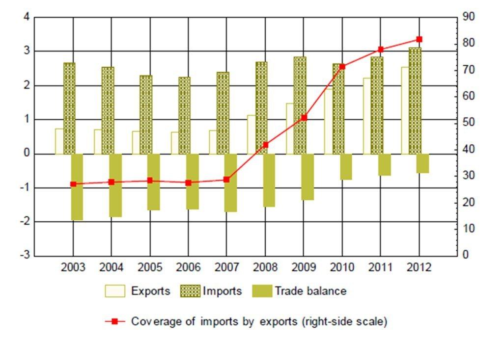
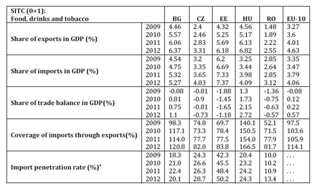
Romania’s trade deficit of food, beverages and tobacco declined markedly from 1.63 percent of GDP in 2009 to 0.75 percent in 2010, mainly due to the substantial dynamics of exports. The trade deficit further narrowed to 0.63 percent in 2011 and 0.57 percent in 2012 (Figure 1). This development was similar to other countries in the region (Table 1).
percent of
percent of GDPpercent
Figure 1: Romania’s food, beverage and tobacco trade balance
Source: Own calculations based on data released byEUROSTAT
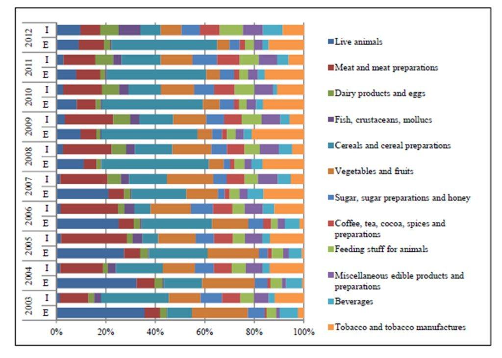
The exports of agricultural products are characterized by a high degree of concentration, the annual change in the physical volume being supported, since 2008, in the proportion of over 73 percent, by four groups of goods: cereal and cereal preparations, meat and meat preparations, live animals and tobacco and tobacco manufactures. The structure of imports of agricultural products shows are duced efficiency of the Romanian food industry that affects the possibility of improvement of the agricultural trade balance. (Figure 2).
Table 1: International trade of food, drinks and tobacco in EU -10 emerging economies
*)… complete data not available for EU-10 countries
Source: Own calculations based on data released by EUROSTAT
Source: Own calculations based on data released byNational Institute of Statistics
Figure 2:Structure of Romania’s external trade of food, beverages and tobacco
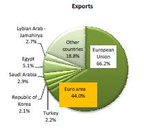
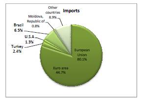
In 2012 the geographical spread shows that EU Member States were the main partners of Romania in trade with food products, beverages and tobacco. Thus, for this category of products, intra-EU exports represented 66.2 percent of the total output and come mainly from the following countries: Italy (13.8 percent), Bulgaria (9.8 percent), Hungary (6.9 percent), Germany (6.5 percent) and Spain (6.4percent). At the same time, intra-EU imports recorded a 80.1 percent share of total inflows, mainly in relation to Hungary (17.9 percent), Germany (13.7 percent), Bulgaria (8.1 percent), Poland (7.8 percent), Netherlands (5.9 percent) and Italy (5.7 percent).

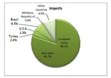
Figure 3: Romania’s trade of food, beverages and tobacco by main partner countries in 2012
Source: Own calculations based on data released byNational Institute of Statistics
With the EU accession of Central and Eastern European countries regional specialization can disadvantage in terms of presence on international markets small economies and those with less diversified economic structure or that are specialized in the export of agricultural products. Introduction of European standards on agriculture, the norms that favour intensive agriculture and limit the production of certain traditional agricultural goods, is expected to have a negative impact in countries with a tradition of small-scale agricultural production, a risk that is still not covered so far.
The econometric model
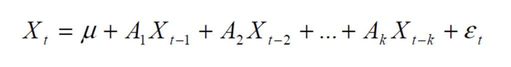
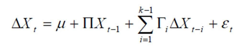
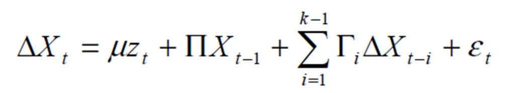
In this study we used the methodology introduced by Johansen and Juselius (1990) to test the co-integration vectors for multivariate models-in which all variables are addressed simultaneously and in order to explain the behaviour variable by its past and that of the other variables. The Johansen test consists in estimating a VAR model including both variables in first differences (assuming that the variables in levels are I(1), and also varying levels (nonstationary taken separately). The matrix of the coefficients attached to the variables in levels contains information on the long-run properties of the model. The Johansen methodology is based on the following p-dimensional VAR with k lags:
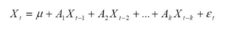
Where Xt is the dependent variables vector (px1), (pxp) coefficient matrices, is the vector of errors or disturbances (px1).
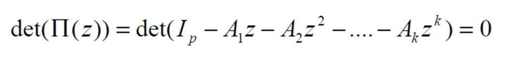
If the equation:
has roots inside the unit circle then some or all variables in vector are non-stationary I(1), and there may be co-integration relationships between them.
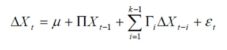
If the component series of vector Xt are stationary in their differences, the model in levels can be rewritten in a form of error correction:
 where:
and
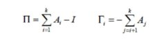
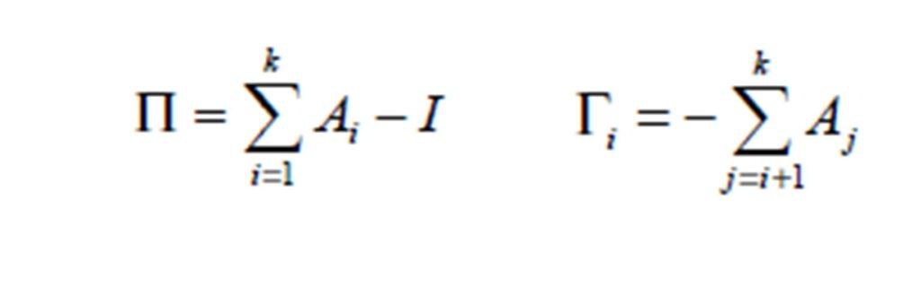
Coefficients contain information on short-run adjustment. Under the co-integration hypothesis, the Î matrix contains information on the long-run relationship between the variables of vector Xt. The rank of the Î matrix indicates the number of co-integration relationships between the p variables in vector Xt. If the matrix has a reduced rank1 ≤ r ≤ p-1, it can be decomposed into matrices α and β of pxr order with rank (α) = rank (β) = r so that Î =αβ’ and β’Xt is I(0), where β is the co-integration vector matrix (r co-integration vectors, each column representing the coefficients of a co-integration vector) and α is the matrix of the adjustment coefficients in the vector error correction model. To determine the number of co-integration relationships the eigen values (or characteristic roots) of the matrix are estimated: These eigen values are equal to the square of the canonical correlation between ΔXt and Xt-1corrected by the ΔXt-I differences, so that they take values between 0 and 1. The number of eigen values significantly different from zero indicates the number of co-integration relationships. The rank of the matrix equals the number of nonzero eigen values. Johansen and Juselius introduced two LR tests (likelihood ratio) to determine the rank of the Î matrix:
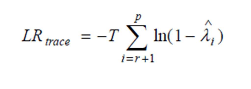
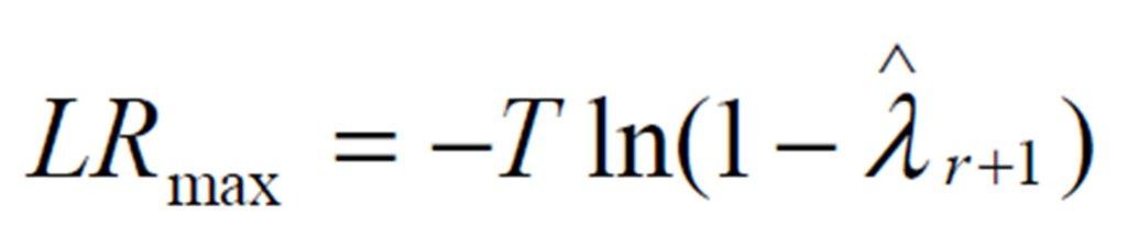
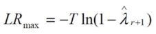
1. The trace test tests the null hypothesis: “there are at most r co-integrating relations” against the lternative of “p co-integrating relations” (i.e., the series are stationary), r=0,1,…,p-1: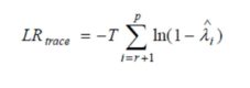 2. The maximum eigen value test tests the null hypothesis: “there are r co-integrating relations” against the alternative “there are r+1 co-integrating relations”:
 The two test statistics do not follow a chi square distribution in general. Asymptotic critical values can be found in Johansen and Juselius (1990). They differ as series have constant and / or deterministic trend and the co-integration equations contain constant and / or deterministic trend. The general form of the model is :
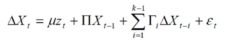
may also include deterministic trends, type t, by the vector of zt deterministic variables.
The validation of the existence of co-integration relationship implies only the existence of the correlation, without providing information about the direction of the causal relationship between the variables. Examining the direction of causality involves carrying out exogenous block tests for each equation in the VECM.
Data description and assessments of the results provided by the econometric model
In the present study, we intend to econometrically quantify the relationship between the determinants and the Romania’s imports of agricultural products. We included the following series of quarterly data into the empirical estimates:
– Imports of agricultural products, millions of lei, average prices of 2000. Source: National Institute of Statistics (IAP);
– Domestic absorption, millions of lei, average prices of 2000. Source: National Institute of Statistics (DA);
– RON/EUR exchange rate. Source: National Bank of Romania (E).
The estimates are based on data from the interval 2003Q1-2012Q4. The imports of agricultural products we deflated by unit value indices of international trade and all the components of domestic absorption (final consumption, gross fixed capital formation and change in inventories) we deflated by the corresponding price indices. The three variables were transformed into natural logarithm, being noted with: IAP, DA, E. The existence of a significant seasonal component was determined for all variables, except RON/EUR exchange rate. We seasonally adjusted the concerned series using the TRAMO/SEATS method.
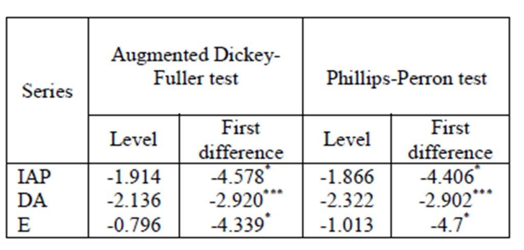
For the three variables included in the study testing the integration order was made through two procedures: the Augmented Dickey-Fuler test and the Phillips-Perron test (Table 2). All variables are integrated of order I, which is consistent with a first difference stationary representation.
The non-stationarity of the series motivated the use of the Johansen multivariate procedure in the analysis to identify the presence of a stationary long-run relationship (co-integration) between non-stationary series. The number of lags used in co-integration is determined by estimating a VAR model. If the VAR has optimal p lags, the VEC will be estimated with p-1 lags. Choosing the optimal number of lags was performed using the criteria of Akaike. The VEC estimated to determine the co-integration relationship included two lags.
Table 2: Tests of Stationarity
*null hypothesis of unit root existence is rejected at the 1% level;
** null hypothesis is rejected at the 5% level; *** null hypothesis
is rejected at the 10% level
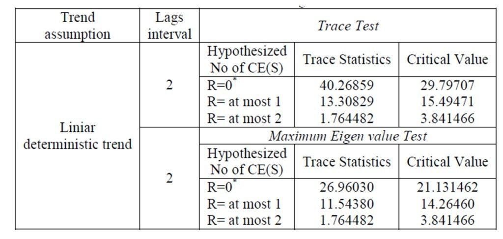
Next, we applied Johansen’s co-integration rank test (Table 3). Both the trace test and the maximum eigen value test show the presence of a single co-integration relationship between the three analysed variables. As regards the diagnosis of residual terms, the results of the tests are satisfactory for the model. With a comfortable margin, the tested hypotheses (lack of auto-correlation, normality and homoscedasticity) are not rejected at the significant conventional levels of 1 percent and 5 percent.
Table 3: Johansen Co-integration Test
*denotes rejection of the hypothesis at the 0.05 level
The obtained co-integration relationship is displayed bellow (standard errors are in parenthesis):
IAP = -16.9577+ 2.0527*DA + 1.5745*E
(0.112) (0.222)
In the long term the imports of agricultural products are positively influenced by the growth of the domestic absorption. Also, the imports of agricultural products and the RON/EUR exchange rate are moving in the same direction. The adjustment speed to the long run equilibrium is -0.05 (with t statistics -4.61), which shows that if in the previous quarter the import of agricultural products was higher than the equilibrium level, in the current quarter it will decrease.
The study utilizes impulse response function as a supplementary check of the Co-integration test’s findings. Botel (2005) mentioned that the impulse response function (IRF) describes the effect of a shock administered to a variable on the future values of each variable in the system, following the trajectory of this impact in time, at different moments. IRF is defined as:
, where: the element on row i, column j of matrix ωs identifies the effect of the increase by one unit of variable uj,t at a time moment t on the variable yt+s, in the conditions when the other variables are maintained constant. The most important information provided by FRS is related to the response sign (positive or negative) and the continued effects of various shocks.
Figure 4:IPA responses to structural innovations
(innovation = a standard deviation)
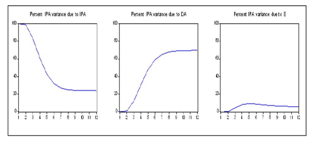
According to the estimated model, we can simulate the impulse response function in the three series as presented in Figure 4. It is noted that IPA responds positively to shocks in the DA. IPA responds negatively to shocks in the E in the first two quarters and then negatively. In addition, IPA responds positively to their innovations. The variance decomposition (VD), on the other hand, provides information on the relative importance of each shock in the hierarchy of the effects on the variables in the system. As the innovations cannot be anticipated, forecast errors are induced in the variables of interest. VD represents a calculation of the share in the total of these variations that is due to shocks coming from each variable.
Figure 5: Variance decomposition of IPA
Going further with the analysis, examining the variance decomposition, it results that after three quarters, the variation of agricultural product imports is 83.42 percent explained by own innovations. On a longer time horizon, the shocks of the domestic absorption and of the RON/EUR exchange rate have an increasing contribution in IPA. These results highlight the difficulties of adapting a relatively stable demand to a variable and hardly modifiable on short and medium term supply. In these conditions, the depreciation of LEU is less accurately reflected in the consumer prices of food products.
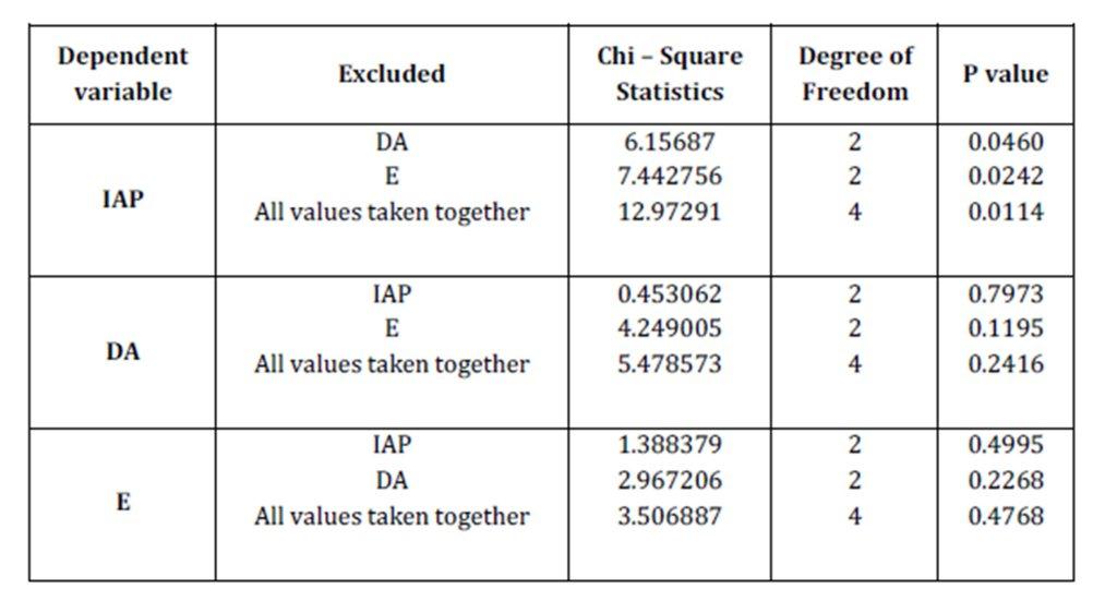
The analysis was continued by applying the Granger causality/ Block Exogeneity Wald Test, whose results are presented in Table 4.
Table 4: VEC Granger causality / Block Exogeneity Wald Tests
We utilized the chi square (Wald) statistics to check the common significance of each of the other lagged endogenous variables in each equation of the model as well for common significance of all other lagged endogenous variables in each equation of the model. As it can be noticed, the results illustrate that DA and E are Granger Causal for IAP at 0.0460 and 0.0242 levels of significance respectively. Also, all the variables are Granger Causal for IAP at the 0.0114 significance level. The null hypothesis of block exogeneity is rejected for the other equations in the model.
Conclusions
The paper examines the causality links between the imports of agricultural products, the domestic absorption and the RON/EUR exchange rate. The co-integration analysis revealed that there is only one co-integrating relationship between the investigated variables. In the long term, the domestic absorption and the imports of agricultural products are moving in the same direction. In addition, the direct relationship between Romania’s imports of agricultural products and RON/EUR exchange rate was recorded due to the existence of a wide range of dysfunctions in the key components of the agricultural food sector: production of raw materials, food industry, and also in distribution and to the high level of self-consumption of rural inhabitants.
Demand for agro-food products is relatively stable, while supply is variable and difficult to change on short notice. From this perspective, knowledge of demand and consumption of agro-food products in our country is absolutely necessary as it: (i) enables those responsible for agricultural and food policies to assess the market potential and to anticipate future developments; (ii) enables farmers and processors to guide their production under structural, quantity and quality features and, therefore, to base their behaviour on the conditions of sale which they anticipate for the future; (iii) directs distributors to choose the structure assortment of the products they will buy for resale to consumers, in the quantity, quality, times and places desired by them.
References
1. Botel, C. (2002) Causes of inflation in Romania, June 1997-August 2001. Analysis based on Structural Vector Autoregressive, Occasional Papers No. 11, National Bank of Romania.
2. Enache, C. (2011) Statistical Analysis of the Sustainable Development Trends in Romania’s Agriculture, Doctoral Thesis, AES, Bucharest.
3. Enders,W. (1995) Applied econometric time series.John Wiley&Sons, Inc.
4. Engle,R.F. andGranger,C.W.(1987) Cointegration and error-correction:representation estimation and testing,Econometrica, vol. 55.
5. Favero, C.A. (2001) Applied macroeconometrics. Oxford: Oxford University Press.
6. Iorga,E., Oancea C. and Stanca R.(2009) The analysis of variance transmission of the industrial production price on the consumer price variation, Occasional Papers no. 26, National Bank of Romania.
7. Johansen, S. (1991) Estimating and testing cointegration vectors in Gaussian vector autoregressive models. Econometrica, 59, 1551—1580.
8. Toderoiu, F.,(2012),” The Romanian Agri-Food Economy — Performance Reductive Effects Five Years of EU Membership”, AgriculturalEconomics and Rural Development Journal, vol.9, issue 1, [Date accessed the site 15.04.2014] Available: http://www.ipe.ro/RePEc/iag/iag_pdf/AERD1201_25-45.pdf
* * * http://epp.eurostat.ec.europa.eu
* * * http://www.bnro.ro
* * * http://www.insse.ro