Introduction
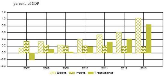
In 2013, the share of agricultural products trade balance deficit stood at 0.32 percent of the GDP, down 0.45 percent points compared to 2007. The coverage of imports by exports was 80.09 percent, 48.08 percentage points more than in2007. The positive dynamics of net exports with developing countries since 2008 contributed to this evolution. In thiscontext, this paper aims to assess the impact of determinants on the imports of agriculture products from the developingcountries by using the Vector Autoregressive Model.
The use of VAR models appeared with works of Sims (1980). He considers that all the variables must be treated as endogenous variables, thus avoiding the corruption of model with identification restrictions that were arbitrarily established (Pauna, 2007). Later on Lutkepohl (1991), Watson, Hamilton (1994), Enders (1995) and Waggoner and Zha (1999) gave updated surveys of VAR techniques. The use of cointegration theory based approaches in the field ofmodelling ensures (Granger-1986, Engle-Granger-1987, Johansen – 1988, Phillips Perron-1988, Johansen şi Juselius-1990, Dickey Fuller-1981) ensures overcoming the problems related to the non-stationary nature of the time series used.
Albu et al (2003) mentioned that applying the cointegration technique allowed the deduction of the long-term equilibriumrelationship, also offering a solid basis for investigating the short-term dynamics. In the last decade the use of this modelhas become an empirical approach that makes sense only if the series included have a long-term relationship, so theyare co-integrated. This means not only that all series are to be integrated by order one and that the residuals to belong to a stationary series, but it also imposes the condition that there should be at least one linear combination of basic series that is stationary.
One of the VAR model characteristics is the fact that it captures the dynamics of several variables simultaneously, and the impulse response functions capture the propagation of the shock of a dependent variable upon the system. Thus, it may answer to very important questions in terms of the economic policy authorities, such as the following one: How do imports of agricultural products react to an innovation in domestic demand?
The study is structured as follows: Section 2 is dedicated to grasping the Romania’s external trade dynamics of agricultural products with developing countries. Section 3 presents the model used. The analysis is based on Vector Autoregressive Model. The data used, the identification method adopted and the actual modelling are described in Section 4. Assessments of the results provided by the econometric model are presented in section 5. The final conclusions are summarized in section 6.
Overall Picture of the Romania’s External Trade of Agricultural Products with Developing Countries
The trade balance of Romanian agricultural products with developing countries has contributed positively to the GDP dynamics since 2008, in terms of a faster pace of export growth compared to imports (Figure 1).
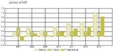
Fig 1: Romania’s Agricultural Products Trade Balance with Developing Countries
Source: Own calculations based on data released by EUROSTAT
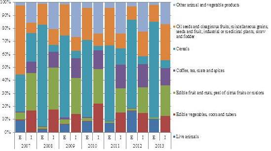
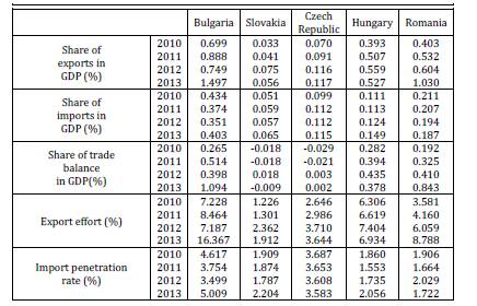
In 2013, the penetration rate of agricultural products imports from developing countries stood at 1.722 percent, substantially lower than the level recorded in other EU countries in the region (Table 1). The foreign trade with developing countries has been characterized by a high degree of concentration, the annual variation in the physical volume for both the exports and imports of agricultural products since 2008 is sustained for more than 62 percent by two and respectively four commodity groups (for exports – cereals and live animals, and for imports – edible fruit nuts, peel of citrus fruits or melons; coffee, tea, mate and spices; edible vegetables, roots and tubers; oil seeds and oleaginous fruits, miscellaneous grains, seeds and fruit, industrial or medicinal plants, straw and fodder (Figure 2).
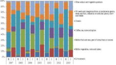
Fig 2: The Structure of the International Trade of Agricultural Products with Developing Countries
Source: Own calculations based on data released by EUROSTAT
Table 1: International Trade of Agricultural Products with Developing Countries – Competitiveness Indicators
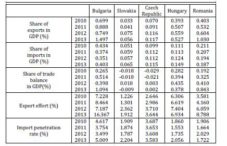
Source: Own calculations based on data released by EUROSTAT
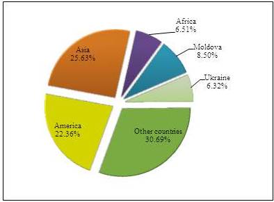
In 2013, 25.63 percent of agricultural products imports from developing countries came from Asian countries, 22.36 percent from Central and South America and 6.51 percent from Africa. The remainder came from Oceania and European developing countries (Figure 4). In terms of exports, the situation is different, the developing states in Africa holding 48.38 percent of the total output in this category of products (Figure 3).
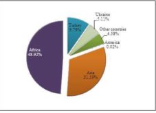

Fig 3: The Geographical Distribution of Fig 4: The Geographical Distribution of
Agricultural Products Exports to Agricultural Products Imports from
Developing Countries Developing Countries
Romania, as an EU member state, supports developing countries to integrate trade into their national developmentpolicies, in programs and strategies to reduce poverty by regulations related to technical assistance for the participationof these countries in the negotiation and implementation of DDA results. In a research study by Zai P.V. (2015) it is mentioned that at the end of 2012, the absorption rate for structural funds in Romania was of less than 6 times higher than in 2009 (11.47 percent), while Lithuania and Estonia were the Central and Eastern European EU Member States with the highest absorption rates — 59 percent, succeeding to attract 4 billion Euros (out of 6.8 billion) — Lithuania and 2 billion (out of 3.4 billion) — Estonia. However, in the period 2007-2013, on average, only 3.67 percent of the total importsof agricultural products from developing countries came from countries of Africa, the Caribbean and the Pacific.
The Econometric Model
In order to highlight the way imports of agricultural products react to various shocks in the economy, we will use a Vector Autoregressive Model, useful in analysing economic policies.
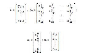
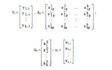
In a research by Pauna (2007) it is considered that the process that generated the time series Yt = (y1t, y2t, …, ynt)’ is the sum between a deterministic trend and a purely stochastic part:
Yt = Ò¹t + xt ,
where Ò¹t is the deterministic part and xt is a zero mean stochastic process. The deterministic component may be zero (Ò¹t=0), may be a constant (Ò¹t= Ò¹o) or may have a linear trend (Ò¹t= Ò¹o+ Ò¹1Ö¼t). The purely stochastic component of process xtincludes the stochastic/co-integration relations trends. It is presumed that it has zero mean and VAR representation. The noticeable process yt takes over the deterministic and stochastic properties from Ò¹t and xt. The integration and cointegration order is given by xt.
It is presupposed that the stochastic part is generated by a VAR process of p order (VAR(p)):
Yt = A0 + A1Yt-1 + A2Yt-2 + … + ApYt-p + ut,
where:
The theory shows that the VAR(p) is stationary if the polynomial defined from determinant det(In-A1Z –…-ApZp) = 0 hasthe roots outside the unit circle in the complex plane (Hamilton, 1994). If the polynomial determinant has a root unit z=1 and all the other roots outside the circle unit, then part of the variables are integrated and there may also be co-integrated variables.
The model can be written in reduced form, in a polynomial way with lag:
A(L) = (In — A1L — A2L2 — … — ApLp)Yt = A0 + ut
or:
A(L)Yt = A0 + ut.
In the case of a VAR process, each series can be estimated by the least square method or by another method (e.g. the maximum verosimility method). The estimated model is written:
Yt = 0 + 1Yt-1 + 2Yt-2 + … + pYt-p + v t
where vt is the dimensional vector (k, 1) of residues.
It is noted with Σv the variance-covariance matrix of residues. The VAR process parameters can be estimated only by starting from stationary time series. Thus, after the study of series characteristics, these are either stationarized by differentiation, before estimating the parameters, in the case of DS series (with random tendency), or a component of trend type is added in VAR specification, in the case of a deterministic trend.
VAR analysis is finalized into three types of results: impulse response function, forecast error variance decomposition and Granger causality.
- The impulse response function (IRF) traces the effect of a shock of a standard deviation of the residuals of a variable on the current values and on the future evolution of all other variables in the model.
- The variance decomposition (VD) provides information on the relative importance of each shock in the hierarchy of the effects on the variables in the system. As the innovations cannot be anticipated, forecast errors are induced in the variables of interest. VD represents a calculation of the share in the total of these variations that is due to shocks coming from each variable.
- The Granger causality (GC) tests reveal what variables are useful for the forecast of other variables. We can state that X causes Granger on Y if a Y forecast made on the basis of a set of information that includes the history of X is better than a forecast that ignores the history of X.
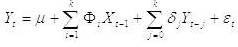
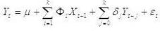
- In order to test whether X is a cause for Y in Granger sense, the regression equation is estimated:
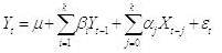
Where k is fixed so that errors are white noise.
The tested hypotheses are the following:
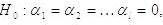
X is not the cause for Y,

The testing of null hypothesis is based on the Fisher-Snedecor test. The null hypothesis is rejected if the value calculated for F statistics is higher than the critical value.
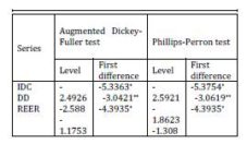
- In order to test whether Y is a cause for X in Granger sense, the regression equation is estimated:
The tested hypotheses are the following:
Y is not cause for X,
The testing of null hypothesis is based on the Fisher-Snedecor test. The null hypothesis is rejected if the value calculated for F statistics is higher than the critical value.
Following the application of the two tests, the following conclusions are possible:
a.Unidirectional causality: X is cause for Y (XY), if the null hypothesis is rejected at i and is accepted at ii;
b. Unidirectional causality: Y is cause for X (Y X), if the null hypothesis is rejected at ii and is accepted at i;
c.Bidirectional causality: XY, if the null hypothesis is rejected both at i and at ii;
d.The two variables are independent if the null hypothesis is accepted at i and ii.
Data Description, Innovation Orthogonalization by the Method Sims Bernanke and the Results of the Diagnosis Analyses for Testing the Statistical Properties
In the present study, I used the VAR technique to assess the factors influencing Romania’s imports of agricultural products from developing countries, using the quarterly data from the period 2007-2013.
The variables, data sources and descriptions used in the econometric estimates are presented below:
- Imports of agricultural products from developing countries, millions of lei. Source: EUROSTAT (IDC);
- Domestic demand, millions of lei. Source: EUROSTAT (DD);
- RON/EUR exchange rate. Source: National Bank of Romania (REER).
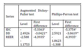
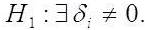
The series are expressed in the average prices of 2005. The imports of agricultural products from developing countries I deflated by unit value indices of international trade, the exchange rate I deflated by CPI and the domestic demand I deflated by the corresponding price index. The existence of a significant seasonal component was determined for all variables. I seasonally adjusted the series using the TRAMO/SEATS method. For the three variables included in the study testing the integration order was made through two procedures: the Augmented Dickey-Fuller test and the Phillips-Perron test. The variables are integrated of order I, which is consistent with a first difference stationary representation (Table 2).
Table 2: Tests of Stationarity
*null hypothesis of unit root existence is rejected at the 1% level;
** null hypothesis of unit root existence is rejected at the 5% level
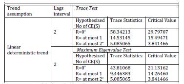
The tests for choosing the number of lags indicate three lags as the optimal number. Using three lags, the VAR becomesunstable, which is why I chose to use two lags. The solution of the characteristic equation indicates a stable VAR. With a comfortable margin, the tested hypotheses (lack of auto-correlation, normality and homoscedasticity) are not rejected at the significant conventional levels of 1 percent and 5 percent. The non-stationarity of series motivated the use of the Johansen multivariate procedure in the analysis, which, by both criteria used, λtrace and λmax, identified, at a statistically significant level of 5 percent, the presence of a long-term stationary relation (cointegration) among non-stationary series (Table 3).
Table 3: Johansen Cointegration Test
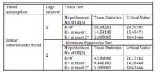
*denotes rejection of the hypothesis at the 0.05 level
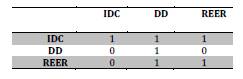
Ortogonalization of innovation or the identification of structural shocks, ut, is made by imposing zero restrictions on the matrix coefficients describing the structural, contemporary relations of the variables of interest (matrix A), using the method Sims Bernanke (1986). The variable in a row is influenced during the quarter by the variables of the columns. “0” means no influence, and “1” indicates the existence of influence. Also, each variable is influenced by itself (Table 4).
Table 4: A Matrix structure
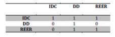
The imposed restrictions indicate that, within a quarter time horizon, the imports of agricultural products from developing countries are affected by the domestic demand and the RON/EUR exchange rate. In turn, the domestic demand influences the RON/EUR exchange rate.
As it can be noted from Figure 5, for both CUSUM test and CUSUM of squares test, the tested indicator chart does not protrude outside the critical band corresponding to a significance level of 5 percent. Therefore, at this significant level, the hypothesis of stable coefficients cannot be rejected, the result giving one more validation to the investigated model.
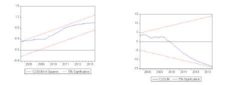
Fig 5: Coefficients Stability Test
Assessments of the Results Provided by the Econometric Model
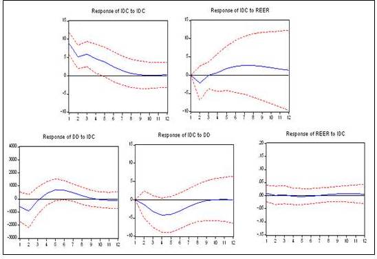
According to the estimated model, I simulated the impulse response function in the three series as presented in Figure 6.
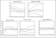
Fig 6: IDC Responses to Structural Innovations
(innovation = a standard deviation)
It is noted that imports of agricultural products from developing countries respond negatively to shocks to the domestic demand and to those coming from RON/EUR exchange rate in the first nine quarters, respectively in the first three quarters and then positively. In addition, the IDC responds positively to the own innovations.
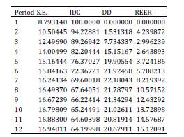
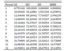
Examining the variance decomposition (Table 5), it results that after four quarters, the variation of agricultural product imports from developing countries is 82.2 percent explained by own innovations. Longer periods of time, the shocks of the domestic demand and RON/EUR exchange rate are much higher, reaching to explain 20.7 percent and 15.1 percent of change IDC after 12 quarters.
Table 5: Variance Decomposition of IDC
% of IDC variance explained by innovations in:
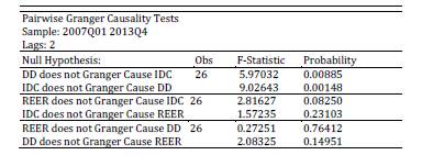
In Table 6 are presented the results of the Granger causality test.
Table 6: The Granger Causality Test
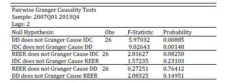
As it can be noticed, the variable domestic demand causes the imports of agricultural products from developing countries in the Granger sense (p-value of the test: 0.00885), therefore the influence of DD has a regular, predictable character. The null hypothesis, according to which the RON/EUR exchange rate does not Granger causes the imports of agricultural products from developing countries, is rejected at 10 percent. In this respect, taking into account the possibility of type I errors, it can say, in the context of the same analysis, that REER is causing IDC, i.e. the value of agricultural imports from developing countries are explained by the past values of the exchange rate and the value of the exchange rate are explained by the future values of the agricultural imports.
Conclusions
The characteristic element of Romanian foreign trade in agricultural products with developing countries is the tendency of continuous growth since 2008 in its proportion in the GDP, also reflecting the economy opening to the outside. The trendof the national economy opening is the result of many factors, among which we mention: the policies for the liberalization of foreign trade, by pronounced as possible opening of the economy to global markets, by the re-division of markets amidthe globalization and regionalization processes.
Throughout the period 2007-2013, Romania registered trade surplus with developing countries in the following product categories: live animals; oil seeds and oleaginous fruits; miscellaneous grains; seeds and fruit; industrial or medicinal plants; straw and fodder and dairy produce; eggs; honey; edible animal products. Export effort gradually increased from 3.581 percent in 2010 to 8.788 percent in 2013. The import penetration rate on the domestic market has fluctuated in the period under review, ranging from 1.664 percent to 2.029 percent.
In the next period, in order to adapt to changes and to increase the competitiveness of the agricultural sector it is necessary to implement a set of fiscal, trade and industrial policies, to allow for the differentiated provision and on limited periods of some facilities to those agents with a relatively high growth potential of the gross value added and of the propagation of technological and innovation progress.
Acknowledgement:
This work was cofinanced from the European Social Fund through Sectoral Operational Programme Human Resources Development 2007-2013, project number POSDRU/159/1.5/S/142115 „Performance and excellence in doctoral and postdoctoral research in Romanian economics science domain”.
References
[1] Albu, L.L, Pelinescu, E. & Scutaru, C. (2003. ‘Modele Si Prognoze Pe Termen Scurt,’ Aplicatii pentru Romania, Expert Publishing House, Bucharest.
[2] Bernanke, B. S. (1986). “Alternative Explanations of Money-Income Correlation,” Carnegie Rochester Conference Series on Public Policy 25.
Publisher – Google Scholar
[3] Binder, M. & Ward, F. (2013). “The Structure of Subjective Well-being: A Vector Autoregressive Approach,”Macroeconomica, 64 (2), 361-400.
Publisher – Google Scholar
[4] Botel, C. (2002). ‘Cauzele Inflatiei in Romania,’ iunie 1997-august 2001. Analiza bazata pe Vectorul Autoregresiv Structural, Occasional Papers No. 11, National Bank of Romania.
[5] Capanu, I., Wagner, P. & Mitrut, C. (1994). ‘System of National Accounts and Macroeconomic Aggregates,’ All Publishing House, Bucharest.
Google Scholar
[6] Chudik, A. & Pesaran, M. H. (2011). “Infinite-dimensional VARs and Factor Models,” Journal of Econometrics, 163 (1), 4—22.
Publisher – Google Scholar
[7] Enders, W. (1995). ‘Applied Econometric Time Series,’ John Wiley&Sons, Inc.
Google Scholar
[8] Engle, R. F. & Granger, W .J. (1987). “Co-Integration and Error Correction: Represantation, Estimation and Testing,”Econometrica, 55( 2), 251-276.
Publisher – Google Scholar
[9] Erceg, C. J. & Linde, J. (2010). “Asymmetric Shocks in a Currency Union with Monetary and Fiscal Handcuffs,” International Finance Discussion Paper No. 1012, Board of Governors of the Federal Reserve System, Washington, D.C., December.
Publisher – Google Scholar
[10] Favero, C.A. (2001). ‘Applied Macroeconometrics,’ Oxford University Press, Oxford.
Google Scholar
[11] Fleming, J. & Kirby, C. (2011). “Long Memory in Volatility and Trading Volume,” Journal of Banking and Finance, 35, 1714-1726.
Publisher – Google Scholar
[12] Granger, C. W. J. (1969). “Investigating Causal Relations by Econometric Models and Cross-spectral Methods,”Econometrica 37 (3), 424—438.
Publisher – Google Scholar
[13] Hamilton, J.D. (1994). ‘Times Series Analysis,’ Princeton University Press, p.259.
[14] Johansen, S. (1991). “Estimating and Testing Cointegration Vectors in Gaussian Vector Autoregressive Models,”Econometrica, 59, 1551—1580.
Publisher – Google Scholar
[15] Johansen, S. & Nielsen, M. O. (2012). “Likelihood Inference for a Fractionally Cointegrated Vector Autoregressive Model,” Econometrica, 80(6), 2667-2732.
Publisher – Google Scholar
[16] Pauna, B. (2007). “Modelarea Si Evaluarea Impactului Investitiilor Directe, Nationale Si Internationale Asupra Pietei Muncii Si Evolutiei Macroeconomice din Romania,” Metode VAR si VEC, Working Papers of Macroeconomic Modelling Seminar 071504, Institute for Economic Forecasting.
Publisher – Google Scholar
[17] Sims, C. (1986). “Are Forecasting Models Usable for Policy Analysis?,” Quarterly Review, Federal Reserve bank of Minneapolis, Winter.
Publisher – Google Scholar
[18] Smith, L. V. & Galesi, A. (2011). ‘GVAR Toolbox 1.1 User Guide,’ CFAP & CIMF, University of Cambridge, Cambridge.
Google Scholar
[19] Zai, P.V. (2015). ‘New Approaches Regarding Structural Funds Absorption — Romania vs. Central and Eastern European New Member States,’ Journal of Eastern Europe Research in Business and Economics, IBIMA Publishing (accepted for publishing).