Introduction
Investigation of the laws of economics using the apparatus of economic theory and mathematics is the domain of a scientific discipline called mathematical economics. The basic method of mathematical economics is creating models of economic phenomena, the so-called mathematic modelling. Mathematization in modelling brings mostly general objective view of the examined phenomena. As a consequence, it thus leads to formalizing the findings and elaboration of new theories, by which it substantially affects the progress within fields. Another advantage of using mathematics in economics is the fact that mathematics is comprehensible to people speaking different national languages. The disadvantage of using mathematics in economics is the risk of the mathematical perspective outweighing the economic one.
Modelling in Economics
Economics is one of the scientific areas within social sciences that focus on business activities of companies and households, cash flow and production systems in the society. When compared to other scientific domains, it is relatively difficult to experiment in a controlled environment and subsequently simulate the specific conditions in which the established theories can be tested. Economists consider models to be a tool that helps them solve particular issues, in a similar way as mechanical engineers creating models to demonstrate how a given system works or biologists using models to illustrate the function of internal organs of living organisms. Models created by observing economic reality and gathering statistical data are mostly based on mathematical disciplines, such as numerical methods, statistics, optimization, linear and dynamic programming, operational research and others. The research in economics includes the process of modelling, analysis, diagnostics, possibly even problem solving by quantitative methods, also followed by regressive economic interpretation and practical application, therefore an adequate computer software is required.
The history of mathematical modelling in the area of economics is very long; it was used at the time when there were no programmable computers or their theoretical concepts. Using computers to solve economic tasks on a larger scale started in the late 1950s when computers became generally available. The main disciplines serving as a basis for mathematical modelling had already been established back then. Yet, the incorporation of computers into the area of mathematical modelling brought a substantial change to mathematical modelling mainly due to the fact that it was possible to abandon the high rate of aggregation (size reduction) of the economic model and its variables, which was otherwise necessary for calculations using traditional numerical mathematics and mathematical analysis. The non-aggregated models enable a more real perception of phenomena existing in the economic reality that is being modelled. The gathered results are immediately applicable to business decision-making and management. Thanks to the massive expansion and improvements in computer technology, particularly computers, the role of models focused on optimization was strengthened. Their computational complexity does not need to be taken into account anymore; all the attention can be directed solely at the core of the problem in question. Besides, computers enabled extensive bodies of statistical data to be gathered, concerning real economic systems that both optimization and descriptive models could be based on. The efficiency and range of software for solving mathematical tasks facilitates solutions of real problems — progress of supply and demand, dynamic behaviour of animal systems, movement in resistance environment etc. The present-day science, mathematics, economics and others cannot function without these programmes anymore.
Dynamic modelling
Mathematical modelling in economics is a field bordering mathematics and economics. When considering a complex economic model, which is hard to solve, often it is advantageous to reformulate this model into a mathematical one, which may not present such demanding solving process. In designing such mathematical model, it is desirable to find sufficient amount of certain principles and relations for given economic variables and thus describe their behaviour. Since economic variables are rarely constant, we must often parametrise via time variable. Such parametrisation is called a function. Frequently, we want to predict how certain variables are going to change, and this is possible thanks to such mathematical models. Modelling of phenomena, which are based on an economic reality and are described by statistical data, is made possible by methods that are primarily based on foundations of mathematical disciplines such as differential calculus (Aluf, 2012; Balasubramaniam, 2014; Faria, 2013),, statistics (David, 2013; Plaček et al , 2013), linear and dynamic programming (Hassan 2011), optimisation (Subagyo, 2014; Zaarour at al., 2014) etc.
Especially dynamic models are characterised by time dependence. In these models, the next state of matter is determined by current states, sometimes even by past states, however never by the future ones. Future state can be found only in very few quantities based solely on the knowledge of the current state of a certain quantity, however it is usually defined by states of other quantities as well. By quantities that should also be expressed in the model, which means that individual quantities are mutually interdependent. Such a model can then represent a system of equations, inequalities, graphs and other links.
In their monograph (1981, p. 42), Kobrinskij and Kuzmin highlighted the necessity for using the variable character of history in dynamic economic models, which influences the system development and leads to significant changes in the nature of the whole process. Simonov in his publications (Simonov, 2003; Simonov, 2009) altered the well-known micro- and macroeconomic models, for example Walras-Evans-Samuelson (WEC) model in regards to supply and demand hold-ups, Allen’s commodity market model (Allen, 1971) taking into account supply hold-ups and demand and offer dependence on the cost and the price rate of change, Vidal-Wolf model (Dychta et al, 2003) of single product sale and others.
Some authors are nowadays coming back to the Kalecki single difference-differential equation model (e.g. (e.g. Asea et al, 1999; Collard et al., 2008).
If we understand time as a continuous variable, we can describe the complex behaviour of monitored quantities by differential equations. By acknowledging not only the current states of a quantity, but its behaviour in the past as well, we can refine a particular model and bring it closer to the reality.
Functional differential equations (FDE) are a suitable tool for the description of such a model, in the form
x(n) (t) =f (t,x(t),..,x(n-1) (t), x(h0(t) ),.., x(m)(hm (t))), (1)
where for the sake of simplification t≥0 and function hi(t) represent argument deformation, most frequently delay. This feature makes these FDE considerably different from the „traditional“ordinary differential equations (ODE). This is the reason why these equations cannot be solved using the standard ODE methods. It is the argument delay that marks the dependence of the modelled variable on the past variable states. The delay can represent a constant as well as delay extent depending on time or the variable value.
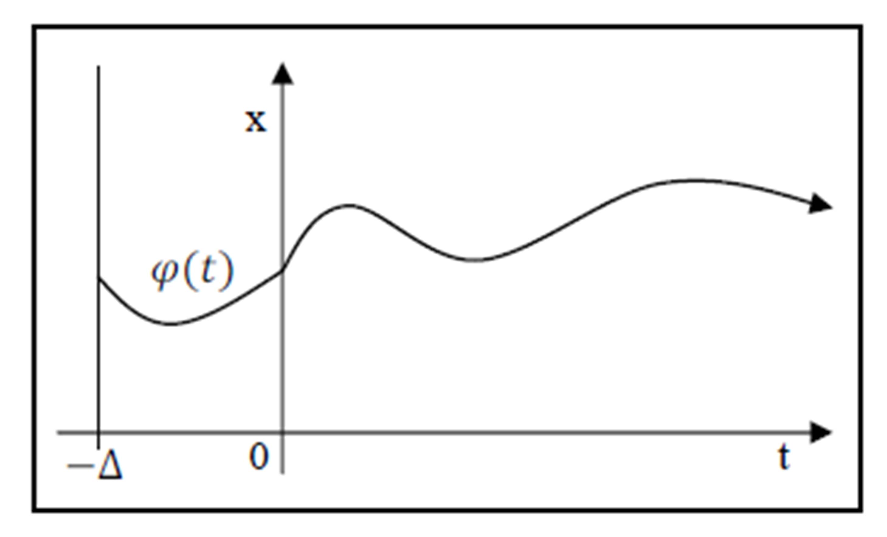
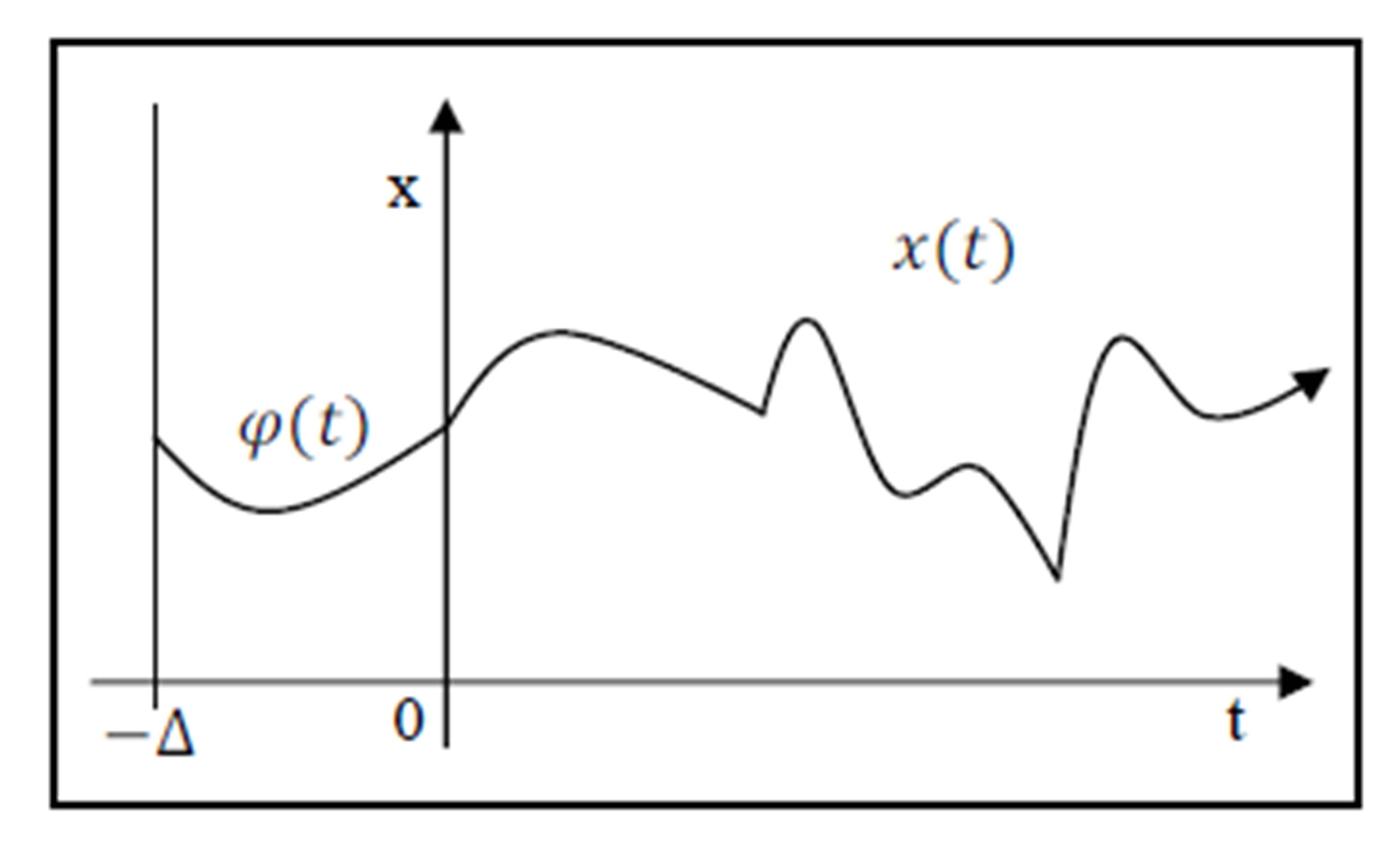
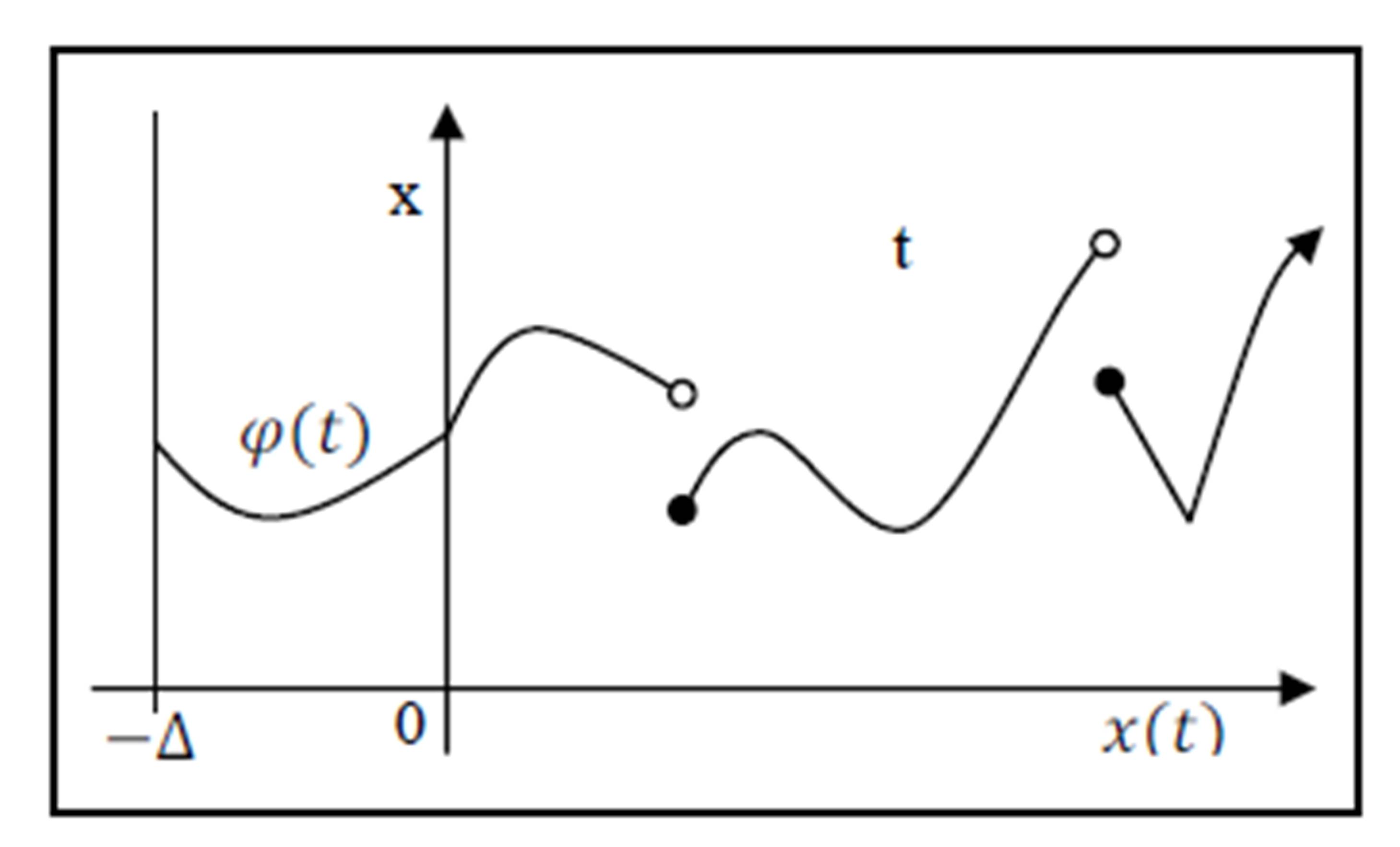
If, as the case often is in applications within economics, the functions hi are a delay, e. g. constant and equal in all components, i.e. hi(t)=t-Δ (where Δ>0 is constant), than the consideration of solving x mathematical model equation needs to be extended by the piece of information concerning the behaviour of the solution in the so-called „initial“ function φ at the interval 〈-Δ,0〉. Then the solution of equation with necessary initial function can be illustrated by the following figure
For the purpose of economic models, the models leading to differential equations and systems complying with Carathéodory’s conditions have proved useful.
Business Management Decision-Making
The above indicated mathematical apparatus will be applied to one of the very significant economic processes, namely inventory use, the objective being the determination of its efficient use.
The area of decision-making processes has become an integral part of all companies. For developing companies, effective decision-making in the conditions of uncertain and unstable external environment is one of the foremost requisites of business success.
A responsible solution of a number of economic issues requires a large amount of appropriately arranged information. On their basis, the decision options have to be determined and the consequences evaluated. Incorrect decisions made on the basis of incomplete or inadequately used information can result in considerable economic losses.
The practical decision-making situations in economics can generally be solved in two ways. The first one, intuitive, is performed based on experience. However, if the intuitive methods and their own experience is not sufficient for the manager, the quantitative analysis methods have to be used.
Company managers have been trying to reduce intuitive decision-making by using different statistical, mathematical and other quantitative methods and thus eliminate the negative consequences of subjective problem solutions in management.
For the solution of economic issues to be efficient and effective, it is necessary to gather and most importantly to adequately arrange the information related to the management and decision-making process. Based on this information, the decision options need to be determined and correctly evaluated and most importantly their results need to be interpreted.
Undeniably, logistics is one of the most important decision-making disciplines in company management. It dates back to the 9th century when it was required for army food supplying and tactics (Drahotský a Řezníček, 2003). However, significant progress came about in the 1940s and during WWII and thus one could say logistics is a relatively young discipline. The findings from this period of progress had significant effects on business logistics, which led to a more in-depth examination of the points at issue, such as the determination of optimum production amount, store placement and efficient distribution (Å tůsek, 2007).
Tangible inventory is one of the key logistics variables. In business management, it is crucial to determine the optimum volume and adjust this value flexibly as necessary in order to minimize the losses resulting from their maintenance.
Inventory is one of the most important elements of current assets, characteristic of their short-term nature. When buying in bulk, the order costs can often be reduced; however, on the other hand the inventory binds a considerable amount of financial resources and thus burdens the economics of the company. Thus inventory is an agent affecting the net income of each company as well as its position in the market, therefore proper attention should be paid to it. High inventory levels reduce the risk of shortage, enable the exploitation of bulk discount and the fulfilment of every contract. On the other hand, they increase both the need of financial resources and the storage costs. Inventory build-up is also usually a signal of imminent financial difficulties.
Despite the undoubtedly positive role of inventory, it is generally considered a manifestation of reserves in the work of managers and there are efforts to decrease their level as much as possible. Since their status is very well measurable and with the current level of computer technology we are able to monitor the inventory status in the supply chains, inventory management is at the centre of attention of specialists in the area of mathematical methods in management.
Model of effective usage of supplies and production
Stock represents the largest investment for many companies. For example, Lambert, et al., 2000 state that the inventory of manufacturing plants may reach over 20% of their total capital and in commercial businesses it may be even over 50%. There is a number of studies that is taking into account aspects of inventory management within the retail environment as well. Their topics are perishability (Bitran et al., 1998; Blackburnet al, 2009), information accuracy (Fleisch a Tellkamp, 2005; DeHoratius, 2008), product range (Ketzenberg et al., 2000), demand substitution (Smith a Agrawal, 2000; Yücela et al., 2009) and bullwhip effect (Novotná, 2015).
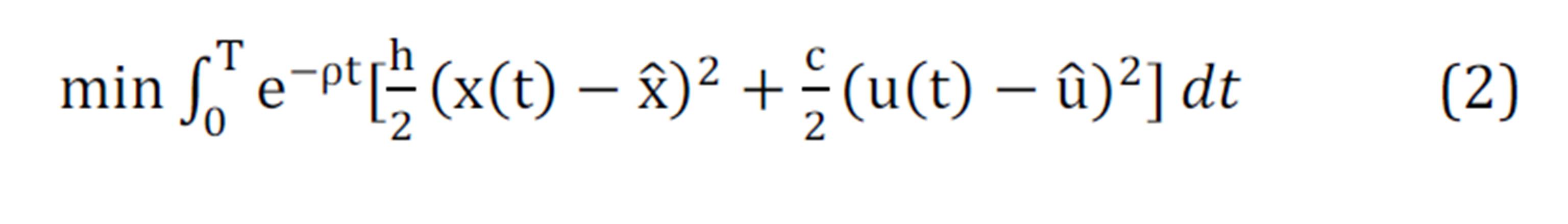
An example of a model using delay differential equations is a system of effective usage of supplies and production (Strelka, 2010). The goal of this model is to minimize the objective function:
where particularly x(t) denote the state of stock in time t, is target state of stock that a company wants to have available, u(t) is the production rate at time t,
  is target production level and s(t) is target rate of sale in time t.
Objective function expresses a certain penalisation for the inefficient use of supplies and productions, which must be minimized in this model by determining the appropriate constants and . It is necessary to identify the optimal size of supplies and level of production. Such valuables are effective only if they can react promptly to changes in demand for a certain product. If a company has large supplies of a product available, it is able to satisfy an unexpected increase in demand for it, however large stocks are also inefficient, because they require financial means that could be otherwise invested for example in securities, to cover the physical storage costs. Vice versa, low product inventory causes loss in profit because of any untraded goods that are not present in stock at the time of increased demand. And thus, deadweight loss effect is formed. Nonetheless, such situations can be effectively addressed via Pontryagin’s maximum principle (PMP) (Strelka, 2010).
The first condition naturally states that change in the stock equals the difference between the sale rate and the production rate. Nevertheless, product manufacturing is not only about the cost of materials that the product is made of, but the time Ï„ that is required for transforming raw materials into the final product as well.
That implies that the first condition can be modified into:
x'(t) = u(t – Ï„) – s(t)
When considering this change, it is necessary to add another initial condition:
u(t) = φ(t), t∈[-τ,0],
where φ(t) is the known nonnegative function within the interval [-τ,0]. Yet, when optimizing the objective function, it is necessary to work with a given delay τ, because in this case the theory of ordinary differential equations is not enough anymore. When dealing with this model via using PMP, the theory of differential equations with deviating argument is subsequently used to achieve the solution.
Conclusion
A number of applications from various scientific fields as well as conclusions provided by theoretical mathematics show that the models based on dynamic relations describe the behaviour of state values very well. The current methods of dynamic system investigation are focused mainly on identifying states in which the system behaves unpredictably, and on identifying states in which the system shows signs of deterministic chaos.
When creating the models, the economists are not presented only with the problem of the theoretical solution of the given problem itself but also with the selection of the tool used to calculate the parameters required for sufficient model description. Delay differential equations can be used in deterministic models, in which it is assumed that all state values are not determined only by the immediate values of the variables entering the solution, but also by their preceding states, at the same time all random influences are ignored.
Acknowledgments
This paper was supported by grant FP-S-15-2787 ‘Effective Use of ICT and Quantitative Methods for Business Process Optimisation’ from the Internal Grant Agency at Brno University of Technology.
References
1. Allen, R. (1971). Matematická ekonomie. (1. vyd., 782, [1] s., Překlad Martin ÄŒerný). Praha: Academia.
2. Aluf, O. (2014). Optimization of RFID Tags Coil’s System Stability under Delayed Electromagnetic Interferences. International Journal of Engineering Business Management, 4(26), pp. 1-15.
3. Asea, P., & Zak, P. (1999). Time-to-build and cycles. Journal of Economic Dynamics and Control, 23(8), pp. 1155-1175.
Publisher – Google Scholar
4. Balasubramaniam, P., Prakash, M., Rihan, F., & Lakshmanan, S. (2014). Hopf Bifurcation and Stability of Periodic Solutions for Delay Differential Model of HIV Infection of CD4 T-cells. Abstract and Applied Analysis, vol. 2014(1), pp. 1-18.
Publisher – Google Scholar
5. Bitran, G., Caldentey, R., & Mondschein, S. (1998). Coordinating Clearance Markdown Sales of Seasonal Products in Retail Chains. Operations Research, vol. 46(issue 5), pp. 609-624.
Publisher – Google Scholar
6. Blackburn, J., & Scudder, G. (2009). Supply Chain Strategies for Perishable Products: The Case of Fresh Produce. Production and Operations Management, vol. 18(issue 2), pp. 129-137.
Publisher – Google Scholar
7. Collard, F., Licandro, O., & Puch, L. (2008). The short run dynamics of optimal growth models with delays. Annales d’Economie et Statistique, 90(1), pp. 127-144.
Google Scholar
8. David, P., Křápek, M. (2013). Older motor vehicles and other aspects within the proposal of environmental tax in the Czech Republic: Other economic indicators. Acta Universitatis Agriculturae et Silviculturae Mendelianae Brunensis, vol. 61(issue 7), pp. 201-219.
9. DeHoratius, N., Mersereau, A., & Schrage, L. (2008). Retail Inventory Management When Records Are Inaccurate. Manufacturing, vol. 10(issue 2), pp. 257-277.
Publisher – Google Scholar
10. Dykhta, V., & Samsoniuk, O. (2003). Optimalʹnoe impulʹsnoe upravlenie s prilozheniiaami. Fizmatlit(1).
11. Drahotský I., Řezníček, B. (2003). Logistika. Procesy a jejich řízení. Brno: Computer Press.
12. Faria, T. (2014). A note on permanence of nonautonomous cooperative scalar population models with delays. Applied Mathematics and Computation, vol. 240(1), pp. 82-90.
Publisher – Google Scholar
13. Fleisch, E., Tellkamp, C., Chen, L., & Mersereau, A. (2005). Inventory inaccuracy and supply chain performance: a simulation study of a retail supply chain. International Journal of Production Economics, vol. 95(issue 3), pp. 79-112.
Publisher – Google Scholar
14. Greguš, M., Å vec, M., Å eda, V. (1985). Obyčajné diferenciálne rovnice. Bratislava: Alfa, vydavateľstvo technickej a ekonomickej literatúry, 1985
15. Hassan, M., Kandeil, A., & Elkhayat, A. (2011). Improving Oil Refinery Productivity through Enhanced Crude Blending using Linear Programming Modeling. Asian Journal of Scientific Research, vol. 4(issue 2), pp. 95-113.
16. Ketzenberg, M. (2000). Inventory policy for dense retail outlets. Journal of Operations Management, vol. 18(issue 3), pp. 303-316.
Publisher – Google Scholar
17. Kobrinskij, N., & Kuzmin, V. (1981). Točnost ekonomiko-matematičeskich modelej. Moskva: Finansy i statistika.
18. Lambert, D., Stock, J., & Ellram, L. (2000). Logistika. (1. vyd., 589 s.) Praha: Computer Press.
19. Novotná, V. (2015). Numerical Solution of the Inventory Balance Delay Differential Equation. International Journal of Engineering Business Management, 7(1), pp. 1-9.
20. Plaček, M. (2013). Utilization of Benford´s Law by Testing Government Macroeconomics Data. In: European Financial Systems 2013: proceedings of the10 th. international scientific conference. (pp. 258-264). Brno: Masaryk University.
Google Scholar
21. Simonov, P. (2003). Issledovanie ustoichivosti rešenij někotorych dinamičeskich modelyach mikro – i makroekonomiki. Vestnik PGTU, 2003(1), pp. 88-93.
22. Simonov, P., & Ustinov, A. (2009). An approach towards quality evaluation of management of budget funds (financial management) in the governmental sector. Vestnik Permskogo Universiteta naucÌŒnyj zÌŒurnal: Economics Series, 2009(1), pp. 63-69.
23. Smith, S., & Agrawal, N. (2000). Management of Multi-Item Retail Inventory Systems with Demand Substitution. Operations Research, vol. 48(issue 1), pp. 319-347.
Publisher – Google Scholar
24. Strelka, M. (2010). Ulohy optimalneho riadenia s ekonomickou motivaciou (Diplomová práce). Univerzita Komenskeho v Bratislave. Fakulta matematiky, Bratislava.
25. Subagyo, E., Aini, N., & Aini. (2014). Good Criteria for Supply Chain Performance Measurement. International Journal of Engineering Business Management, 6(9), pp. 1-7.
26. Å tůsek, J., (2007). Řízení provozu v logistických řetězcích. Praha: C. H. Beck.
27. Yücel, E., Karaesmen, F., Salman, F., & Türkay, M. (2009). Optimizing product assortment under customer-driven demand substitution. European Journal of Operational Research, vol. 199(issue 3), pp. 759-768.
Publisher – Google Scholar
28. Zaarour, N., Melachrinoudis, E., Solomon, M., & Min, H. (2014). A Reverse Logistics Network Model for Handling Returned Products. International Journal of Engineering Business Management, 6(13), pp. 1-10.
Google Scholar