Introduction
The identification of extreme values is particularly difficult in the nonparametric setting where we don’t know the distribution properties of the population under analysis. As noted in Wilson (1993), outliers should be corrected when possible or deleted from the sample so that results don’t get biased. However, extreme values may carry with them important information about the sample of data and their elimination can oversee interesting aspects. Also, outliers are not necessarily amongst the super-efficient units, but can lie inside the interior of the frontier. This particular case can reveal important insights regarding the data.
In nonparametric analysis, it is known that frontiers are particularly sensitive to outliers and results can be highly biased if we don’t take them into account (Daraio and Simar (2007), chapter 5).
An outlier is defined as an element of a set “which is inconsistent with the majority of the data or inconsistent with a subgroup to which the element is meant to be similar” according to Fan et al. (2006). Wilson (1995) defines “outliers are observations that do not fit in with the pattern of the remaining data points”.
Khezrimotlagh (2015) proposed a method to identify outliers in DEA models using Kourosh and Arash method and no other additional complex computations. He also classifies outliers into four categories:
Outliers as outcome from measurement error
As a result of miss selection of inputs/outputs — which can be eliminated by adding a correct input/output
Due to a non-homogeneous DMU (decision making unit) among observations
The Near and Far data type of outliers, which use disproportionate quantities of input /output, in case of, for instance, the use of a much larger quantity of input to produce only slightly more output.
The methodology proposed by Khezrimotlagh (2013) to identify outliers is post analysis, stating that DEA is sufficient to find extreme values.
So there is a double side for outliers as they can be interesting from a statistical point of view or just a measurement error and considered noise for the sample data. Extreme values can also indicate management practices or anomalies in a system’s functioning. In the universities particular case, outliers could indicate abuse in teaching or lack of quality, or even management decisions.
According to Andrews and Pregibon (1978) (AP), the points which have a significant impact on the results are subject to further investigation to see whether they could be outliers. They construct a statistic to identify outliers in a multiple input single output framework by splitting the contribution of each observation to the volume of the full sample data. Later, in 1993, Wilson extends the methodology in AP to multiple output frameworks. Fox et al. (2004) refer to it as the Wilson-Andrews-Pregibon (WAP) measure when comparing it to the methods they proposed based on dissimilarity.
A set of outlier mining algorithms have been developed to identify outliers in different applications. A couple of issues have arisen in relation to these algorithms, one of them is how do we differentiate local from global outliers. Usually a small sample data is available to the researcher and it may be only a cluster of the true population contained in it.
Candelon and Metiu (2013) develop a two stage bootstrap method to identify outliers in a population where no statistical distribution is known, but where univariate data are used.
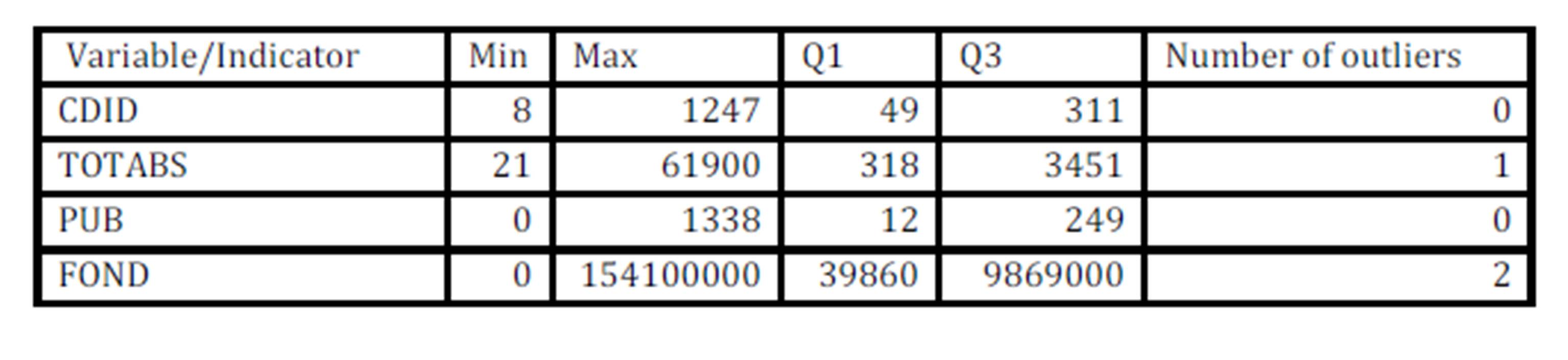
A method of identifying outliers in each set of data corresponding to one variable at a time is based on Tukey’s box-plot method where outliers are found outside the interval: [Q1-1.5IQR; Q3+1.5IQR], where Q means quantile and IQR refers to the inter-quartile interval, as mentioned in Patterson (2012). This is a simple method used to generate immediate outliers for each variable.
Patterson (2012) proposed an algorithm where he divides the set of data into bins where the distance between points in a bin is max ε. The main bin is given by the group with the most elements and any point outside the main bin is considered an outlier.
Detecting outliers using the frontier order-m models proposed by Simar (2003) and based on the idea found in Cazals et al. (2002) can be used to identify extreme values in nonparametric models. In this paper, I use the order-α robust frontier to identify outliers proposed in Daouia and Simar (2007) and implemented in the software package frontiles in R. I am not aware of any other study to apply this method in an empirical application, so this analysis contributes to the evidence of this method’s usefulness in identifying outliers for nonparametric models.
The next section briefly presents the methodology used in the analysis, followed by the description of the sample data. Models and results are explained in the Results section. Conclusions come at the end.
Methodology
As Daraio and Simar (2007) point out, the order- partial frontiers are more robust to extreme values since they do not envelop all the data points, but only a fraction of them. Therefore, I can use the partial frontiers in order to identify outliers using the procedure below (which was first proposed by Simar (2003) for the order-m frontiers). Although the two types of partial frontiers (order-m and order-α ) are different except for the case when m tends to infinite and α score tends to one Daouia and Simar (2007), I can use the same logic explained in Simar (2003) to find the outliers in the probabilistic setting.
In this respect, the procedure applied in this paper assumes the construction of partial frontiers for different values of the parameter α and observe the points which remain outside the curve. If there are DMUs which remain outside the frontier even for high percentages, I have an indicator for possible outliers. The order-α frontier is more robust to outliers than its counterpart order m partial frontier for the same sample data (Daouia and Simar, 2007).
The values for the α parameter (the percentage of points taken into consideration for comparing efficiency) are chosen such that I can observe the changes in frontier orientation and the graphical visualization has proved to be very useful.
In order to decide what value of the parameter α is considered high enough to define it as a threshold for outliers, I plot the number of units outside the frontier for each value of the parameter. Observing the shape of this curve, I can make an educated guess when the line becomes smooth enough as to no serious variations are to be expected in the number of units.
It is fair to assume that a university aims at maximizing the results or the outcome of research or teaching when limited input resources are available. Most of the time, funding or human capital are not the objective of minimization even if we had a price associated with each of them. Therefore, all models are run in the output orientation.
Data description
The data used were gathered from an evaluation study made by the Ministry of Education and Research in 2011 in Romania to evaluate the higher education institutions. The database contains 89 universities and reports on four variables for the academic year 2008-2009 described below:
Results
Several scenarios have been run so that I can include different models with one input and one output variables.
After running a sensitivity analysis, I decided to use values for the α parameter ranging from 0.90 to 0.99, indicating a minimum inclusion of 90% of the observations. The data set is not particularly high (only 89 observations), so I don’t want to eliminate more than the necessary. As a rule of thumb, up to a fraction of can be eliminated, meaning 10% for our case. For the computations and the graphical representation, I used package frontiles developed in R by Daouia and Laurent (2013) updated on 19 of Feb, 2015.
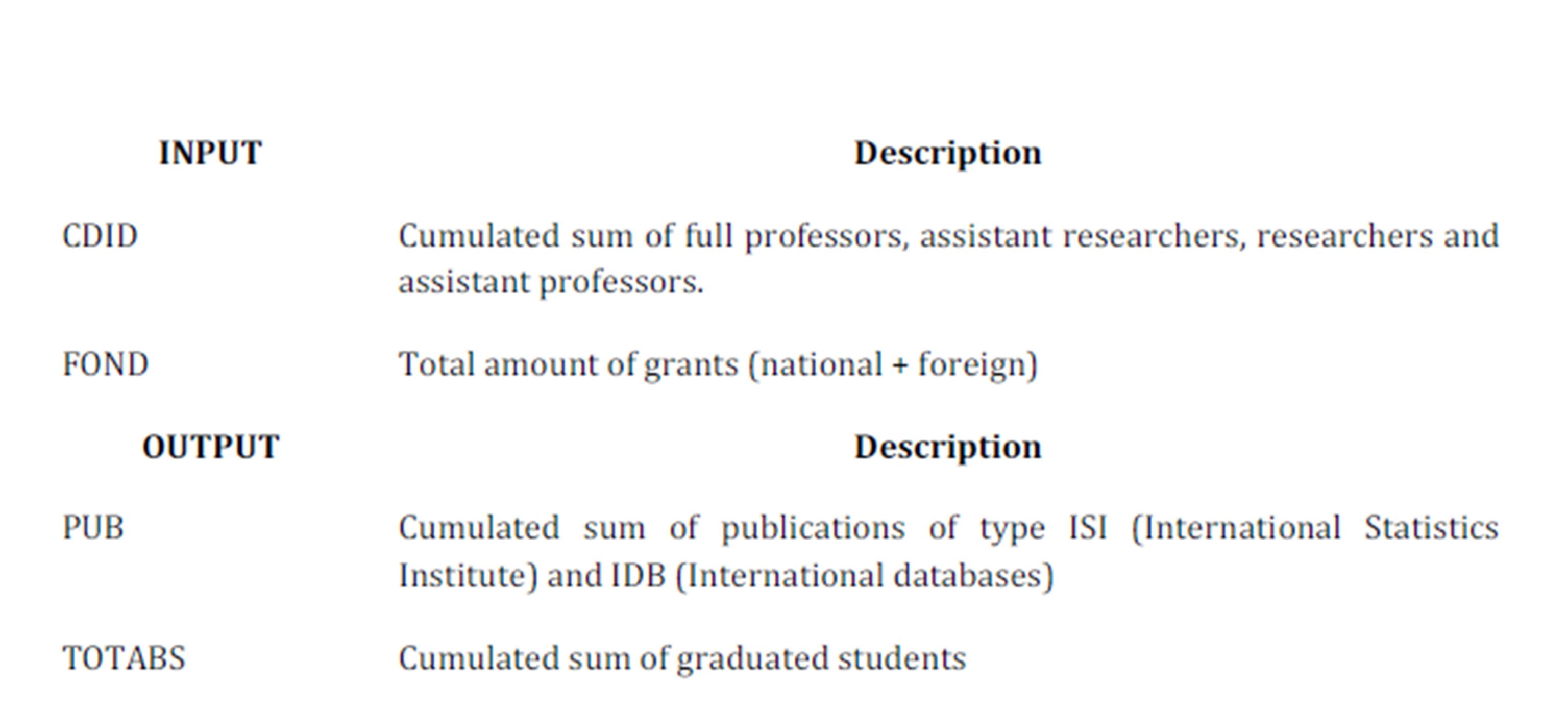
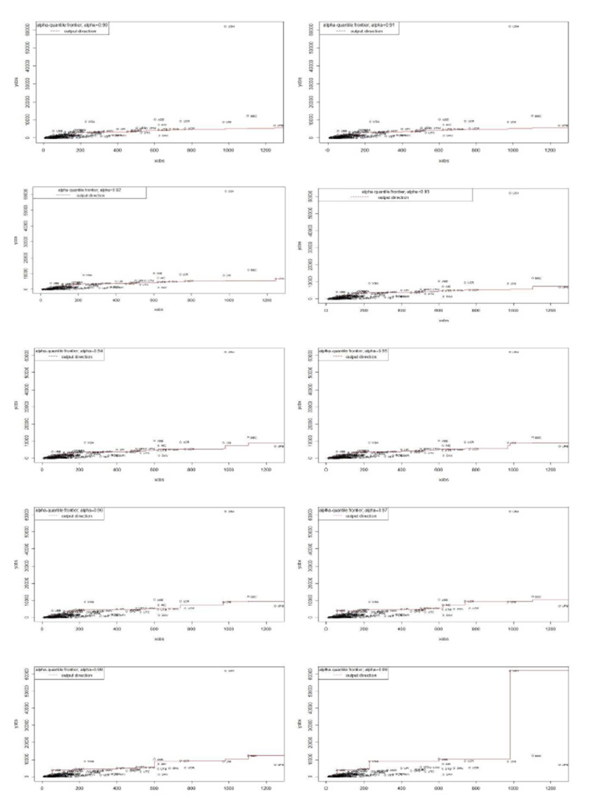
Scenario 1: Representing partial frontier in 2D using the model one input: academic staff -> one output: total graduates.
As it can be seen in Figure 1, the shape of the frontier is similar in the first nine graphs but changes significantly in the last graph, where I include 99% of the observations. University Spiru Haret in Bucharest remains outside the partial frontier even for high values of parameter α. Only when 99% of the universities under analysis are considered for the frontier, this university is also enveloped. Because the shape of the curve is very different in this last graph and only because of this last university, I can say that the DMU is an outlier for this scenario.
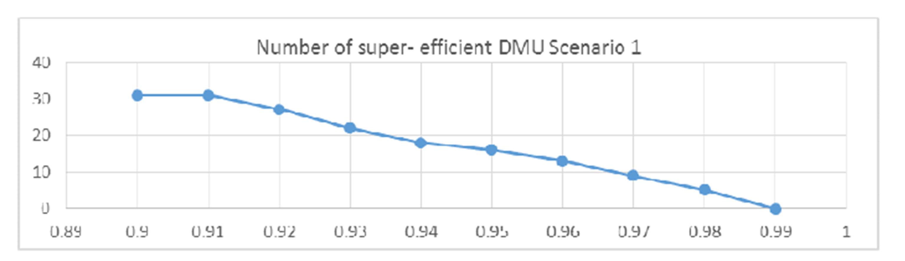
Scenario 2: Representing partial frontier in 2D using the model one input: academic staff -> one output: publications.
In this case (Figure 2), even when I increase the value for the α parameter, the shape of the frontier does not significantly change. The modification which takes place includes translations of the frontier to the left upper side to include observations more and more efficient, but the general shape is similar. For this reason, I cannot conclude on the existence of any outlier in this scenario.
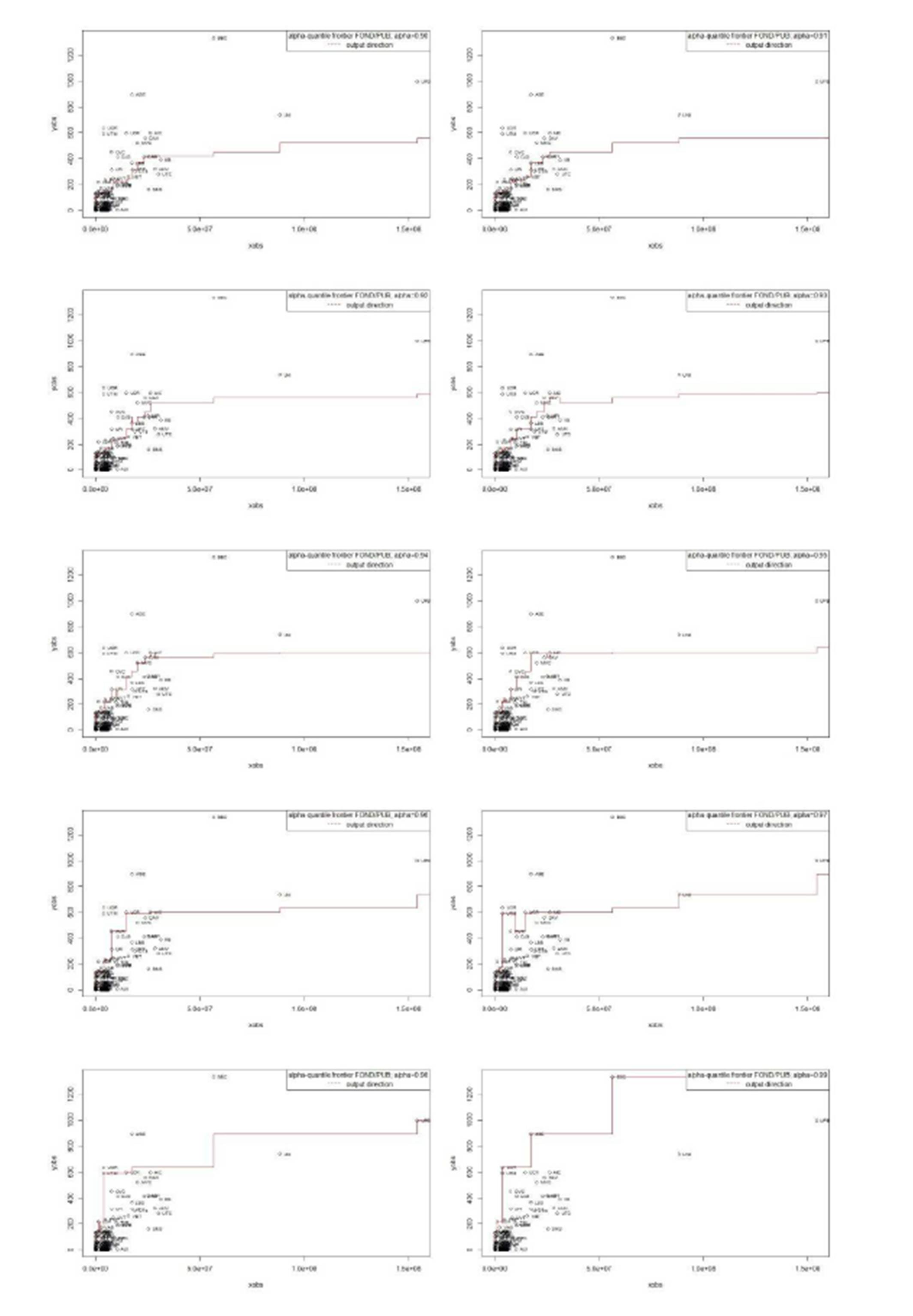
Scenario 3: Representing partial frontier in 2D using the model one input: financial funds -> one output: total graduates.
For this model, I have a similar situation to scenario 1. For high values of the α parameter, 0.98 and 0.99, the shape of the frontier changes significantly when University Spiru Haret is included. This indicates a possible extreme value for this DMU in this scenario as well.
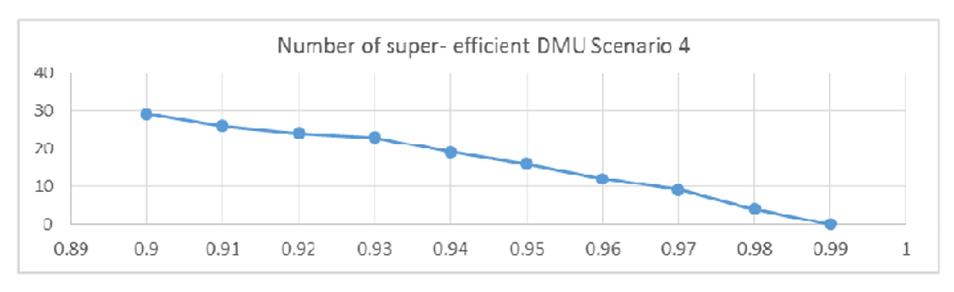
Scenario 4: Representing partial frontier in 2D using the model one input: financial funds -> one output: publications.
For this model, the efficient frontier changes shape by translations, but no significant modification can be observed. In this case, I cannot clearly identify an outlier. It seems that in case I include the research output into the model, there is no clear indication for extreme values. However, in case of graduates, universities are more likely to induce outliers, if we think about the quality of teaching.
The analysis of correlation between the number of DMUs which remain outside the partial efficient frontier and the trimming parameter is presented below for each model:
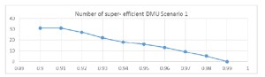
Figure 1 Number of super efficient DMUs for parameter α variable – Scenario 1
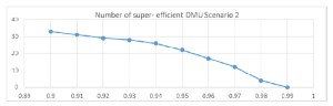
Figure 2 Number of super efficient DMUs for parameter α variable – Scenario 2
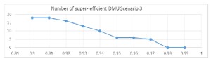
Figure 3 Number of super efficient DMUs for parameter α variable – Scenario 3
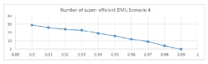
Figure 4 Number of super efficient DMUs for parameter α variable – Scenario 4
From the analysis above, I can only point out in model 3 a clear indication of a smooth inclusion of all units for parameter value greater than 0.98. For the other charts, all differences from one value to the next one are quite smooth and I cannot state clearly when I have a significant change in the number of excluded units.
For comparison reasons, let’s assume we want to find outliers using a simple method for each of the variables in the data set. Then we can use Tukey’s box-plot method of identifying outliers presented in Patterson (2012) which assumes outliers are values outside [Q1-1.5IQR; Q3+1.5IQR], where IQR is the interquartile range. I adapted the range to our data to find the parameter value of 5 to be suitable. The range is then considered [Q1-5IQR; Q3+5IQR].
The analysis for the four variables is summarized below:
Table 1: Summary of Tukey’s box-plot method results
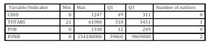
We found one outlier for total graduates in University of Spiru Haret in Bucharest with a value of 61.896 for the number of graduates. I also found two outliers for the financial funds with extreme values for University of Bucharest with a total amount of grants of 88.297.047 RON and Polytechnic University of Bucharest with a value of 154.140.452 RON. The decision to exclude or not those outliers from the analysis is in the hands of the analyst, but excluding them we can oversee some important aspects of the data. It can be that those DMUs are super-efficient, but they can also reveal facts about the institutions’ management.
Conclusion
The paper provides an empirical illustration of the method of identifying outliers first proposed by Simar in 2003 and adjusted for the probabilistic setting. Different scenarios are run according to various one input one output efficiency models. The analysis includes a summary of a nonparametric method of identifying outliers and an empirical illustration for universities data.
The technique can be applied as a preliminary analysis for an empirical nonparametric application.
Results show that sensitivity analysis related to the different values of the parameter α can reveal important modifications in the shape of the robust frontier. Potential extreme values remain outside this curve even when almost all observations are taken into account.
We also applied the Tukey’s box-plot method of identifying outliers for each variable under analysis to identify extreme values at a univariate level. I found one outlier common to both techniques: University of Spiru Haret in Bucharest.
Further analysis can be done to include the “quality” of teaching dimension in the analysis to be able to point out if this university is indeed lacking quality when teaching or it is a super-efficient observation holding rather interesting insights.
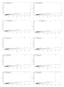 Figure 2 Scenario 1

Figure 4 Scenario 3
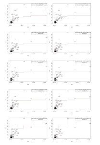
Figure 5 Scenario 4
Acknowledgement
This work was supported by the project “Excellence academic routes in doctoral and postdoctoral research READ” cofunded from the European Social Fund through the Development of Human Resources Operational Programme 20072013, contract no. POSDRU/159/1.5/S/137926.
References
1. Andrews, D. F., and Pregibon, D. (1978). Finding the Outliers That Matter. Journal of the Royal Statistical Society, Ser. B, 40, 85- 93.
2. Candelon, B. and Metiu, N. (2013). A Distribution free test for Outliers. Deutsche Bundesbank Discussion paper. no 2/2013. [Online], [Retrieved Jan, 10. 2015]. https://www.bundesbank.de/Redaktion/EN/Downloads/Publications/Discussion_Paper_1/2013/2013_02_01_dkp_02.pdf?
__blob=publicationFile.
3. Cazals, C., Florens, J., & Simar, L. (2002). Nonparametric frontier estimation: a robust approach. Journal of Econometrics, 106, 1—25
Publisher – GoogleScholar
4. Daouia, A, Laurent, T. (2013). Partial Frontier Efficiency Analysis. [Online], [Retrieved Feb, 19. 2015]. http://cran.r-project.org/web/packages/frontiles/frontiles.pdf
5. Daouia, A and Simar, L. (2007).Nonparametric efficiency analysis: A multivariate conditional quantile approach. Journal of Econometrics. 140. 2007. Pp 375-400.
Publisher – GoogleScholar
6. Daraio, C. and Simar, L. (2007). Advanced Robust and Nonparametric Methods in Efficiency Analysis. Springer US. New York, USA.
GoogleScholar
7. Fan H., Zaiane, O.R., Foss, A. and Wu, J. (2006). A nonparametric outlier detection for effectively discovering top-n outliers from engineering data. PAKDD 2006. LNAI 3918. pp. 557-566. Springer-Verlag Berlin Heidelberg 2006.
Publisher – GoogleScholar
8. Fox, K., J., Hill, R. J. and Diewert, W. E. (2004). Identifying outliers in multi-output models. Journal of productivity Analysis 22 (1-2), 73-94.
Publisher – GoogleScholar
9. Khezrimotlagh, D. (2015). How to detect outliers in data envelopment analysis by Kourosh and Arash method. . [Online], [Retrieved Feb 2, 2015]. http://umexpert.um.edu.my/file/publication/00013084_118960.pdf .
GoogleScholar
10. Patterson, N. (2012). A robust, non-parametric method to identify outliers and improve final yield and quality. CS Mantech Conference, April, 2012. Boston, Massachusetts USA.
GoogleScholar
11. Simar, L. (2003). Detecting outliers in frontier models: a simple approach. Journal of Productivity Analysis, 20, 391—424.
Publisher – GoogleScholar
12. Wilson, P. W. (1993). Detecting Outliers in Deterministic Nonparametric Frontier Models with Multiple Outputs. Journal of Business and Economic Statistics. July 1993, Vol. 11, No. 3, pp 319-323.
Publisher – GoogleScholar
13. Wilson, P. W. (1995). Detecting Influential observations in data envelopment analysis. Journal of Productivity Analysis. April 1995, Vol. 6, Issue 1, pp 27-45.
GoogleScholar