The Relationship between Two Return Rates as a Basis for Performance Evaluation

Introduction

It is known that return rates represent the most popular instruments of measuring the economic and financial performances of companies. If one follows the dictionary definition of the performance, one can find that this term refers to obtaining results in one specific area (Vâlceanu et al., 2004). However, in the economic field, this word is often referred to profitability, productivity and return (Vâlceanu et al., 2004).

As for the aspects noted above, if the return is a form of measuring the performances, one can say that two of the most popular return rates are: return on used resources and return on sales and these are calculated considering the profit and loss statements.

The objective of this work refers to analyzing the correlation between the two previously mentioned return rates.

The methodology used in order to achieve the specified goal refers to the correlation method and to the bibliographic research. The first is used when between the analyzed objective and the influencing factors there is at least one stochastic relationship (Vâlceanu et al., 2004). The second method is used for defining the area studied and is presented especially in the literature review chapter.

It is known that the empirical research or the method of correlation means to accomplish several stages: formulating the hypothesis, choosing the data sample, finding the best econometric model, estimating, testing and validating the model, obtaining and interpreting the results.

Overall, the proposed study comes to establish whether there is any correlation between the two mentioned rates, for Petrom and Zentiva companies, as these results are useful for both the literature in the area and for the two companies, which can assess their future strategies based on the results found. More than that, it is always useful to have a study from which further analyses could start, as no clear evidence on this issue is available as far as I know.

This study is structured as follows: a short review of the specific literature, the development of a hypothesis, the econometric study, the results and the conclusions.

Literature Review

The concept of economic and financial performance as of the existing specific literature refers to returns which usually take into consideration the results obtained based on inputs utilization, that are the elements presented in the profit and loss statement (Vâlceanu et al., 2004).

The return is defined as the ability of a company to obtain profits by inputs and capital utilizations (Vâlceanu et al., 2004). The return is a synthetic form of expressing the efficiency of a company’s activity, which is of all inputs used, bearing in mind all the economic cycle stages: supply, manufacture and sale (Vâlceanu et al., 2004).

In the specific literature, several researchers have analyzed the economic and financial performance through the return rates, especially using the return on assets and the return on equity for various situations or for different companies that have operations in a particular area. For example, Shim (2011) analyzes if the financial performances of companies measured using the return on assets and the return on equity increase or decrease in the specific case of a merger or acquisition of companies (Shim, 2011).

Another interesting study regarding the performance of merged companies is that of Hagendorff et al. (2009) that explore the operational strategies adopted by banks in the United States compared to those adopted in Europe, using accounting data for the comparison of long term performances of acquisition strategies (Hagendorff et al., 2009).

For examining the implications of merged banks profitability, there are put into discussion the changes of OPCFROA indicator (Hagendorff et al., 2009). This indicator refers to the cash flow before taxation related to the historical value of the assets, where the cash flow before taxation is computed as the sum of income before taxation and exceptional elements and loans expenses (Hagendorff et al., 2009). The OPCFROA indicator includes two types of interest expenses for banks: interest expenses that result from the financing decision and those from the financial mediation (for example the interest paid for deposits) (Hagendorff et al., 2009). By contrary, the accounting indicators that consider the earnings (for example the return on assets and the return on equity) include general interest expenses which are influenced by the merger accounting method and by the merger financing method (Hagendorff et al., 2009).

Considering the above aspects, the performance measurement using the accounting data as instrument is one of the most objective evaluation methods of the companies’ success. The researchers from this area have as an argument the business strategic scope of obtaining satisfactory returns (Papadakis et al., 2010).

Although the studies based on the accounting information have not just a few advantages, one can say that there are also disadvantages of using this method (Papadakis et al., 2010). First of all, the accounting profits represent the most limited performance measurement method due to the fact that they measure only the economic performance of a company (Papadakis et al., 2010). Furthermore, the performance measurement using accounting refers only to reflect the past performance of a company (Papadakis et al., 2010).

Two return rates less common for the specific literature are the return on used resources and the return on sales.

The return on used resources reflects the relationship between the profit corresponding to the turnover and the total costs of selling (Vâlceanu et al., 2004). Considering the reference to the operational activity, this rate is calculated by reporting the operational result to the operational expenses or by reporting the profit that corresponds to the net turnover to the expenses corresponding to the net turnover (Vâlceanu et al., 2004).

The return on sales shows the efficiency of a company’s commercial activity by expressing the liaison between the profit and turnover (Vâlceanu et al., 2004). This rate is calculated by reporting the profit (net, corresponding to the net turnover or operational) to the net turnover (Vâlceanu et al., 2004). The most important limit of this rate in defining the performance is generated by the fact that it is calculated on the basis of the accounting profit and in this way the rate will be influenced by the accounting politics and practices used by companies, that are the methods of depreciation of fixed assets, the methods of inventories evaluation, the supply politics, etc. (Vâlceanu et al., 2004).
Because there are no clear evidences of an analysis of the two rates in the specific literature, I propose a study of the possible correlation between these rates, starting from the fact that often in the specific literature the companies’ performances may be analyzed using the return indicators, that are calculated based on the accounting data, that information is from the profit and loss statement.

The Hypothesis Development, the Econometric Model and the Variables

As widely known, the return on used resources and the return on sales have the advantage of being calculated using only the profit and loss elements, without being necessary additional information as that from the management accounting (Vâlceanu et al., 2004). Considering the computing methods and the possible relationship between the two rates, I propose as a hypothesis the existence of a correlation between the return on used resources and the return on sales.

As far as I know, the approach of these two return rates is not common in the specific literature. Nevertheless, the two indicators have a particular relevance for the performance analysis.

The proposed econometric model is as follows:

Return on used resourcesi = a + b * return on salesi + xi, i = 1,…, n
where, Return on used resourcesi is the objective variable;

Return on salesi is the independent variable;

xi represents the residual variable;

n represents the number of considered quarters / semesters.

The above hypothesis refers to the fact that the return on used resources is correlated to the return on sales for the companies’ consideration in the data sample chapter.

Research Methodology

Data Sample

For testing the hypothesis previously defined, the selection of the companies was based on several criteria: the companies have been listed, they have had activity on the Romanian market and the accounting information has been available on the companies’ internet sites. Analyzing a couple of organizations, the ones that were considered as data sample are Petrom and Zentiva. Both companies have operated on the Romanian market: the gas and oil industry (Petrom) and the pharmaceutical industry (Zentiva).

Petrom has an interesting history. It has been established in 1991 as Regia Autonomă a Petrolului PETROM S.A. (Petrom, 2012). In 2004, the Austrian company OMV has acquired 51% of Petrom’s share capital and in January 2010, the company’s name was changed into OMV PETROM S.A., as a consequence of the General Meeting of Shareholders’ decision of 20th of October 2009 (Petrom, 2012). However, the name of the trade mark and logo of the company remained the same (Petrom, 2012).

The shareholders structure of Petrom is: 51,01% OMV AG (OMV Aktiengesellschaft), 20,64% the Romanian Ministry of Economy, 20,11% Fondul Proprietatea S.A., 2,03% EBRD (European Bank of Reconstruction and Development) and 6,21% private investors (Petrom, 2012). In 2001, Petrom was listed at the Bucharest Stock Exchange and the first date of shares trading was 3rd of September (Petrom, 2012).

Zentiva has a long history. The history has its roots in 1962 when it was established as a company of drugs manufacturing (Zentiva, 2011). This company was part of the state system which provided drugs to the internal market (Zentiva, 2011). Later, the company’s name changed into Bucharest Medicines Plant and in 1990 it was called Sicomed (Zentiva, 2011). In 1998, the company was listed at the Bucharest Stock Exchange, its shares being ones of the most sought after at that moment (Zentiva, 2011).

In 2005, Zentiva acquired Sicomed (Zentiva, 2011). In the first semester of 2006, Zentiva integrated the past activities of Zentiva group on the Romanian market with the existing ones of Sicomed (Zentiva, 2011). Zentiva becomes the leader on the Romanian market for general drugs (Zentiva, 2011).
The shareholders structure of Zentiva at 4th of June 2010 was: 50,9809% Venoma Holdings Limited, 23,9282% Zentiva NV, 6,6842% Sanofi-Aventis Europe, 9,6417% other legal persons, 8,7650% individuals (Zentiva, 2011).

The data selected for Petrom refers to the period between the second quarter of 2004 and the fourth quarter 2009 due to the fact that before the second quarter 2004 there was no available information on Petrom’s internet site. The data for the period after the fourth quarter 2009 was eliminated from the data sample because, starting with 2010, Petrom reports its quarterly consolidated results in accordance with the International Financial Reporting Standards (Petrom, 2012). Petrom’s statements of individual results are elaborated in accordance with the Romanian Accounting Standards, but starting with 2010 these are available only for semesters and annual periods of time (Petrom, 2012).

Information for Zentiva was selected for the period between the first semester 2004 and the first semester 2011. Although initially I considered quarterly periods of time, there was no sufficient available data for each quarter on Zentiva’s internet site. Also, the information previous to the first semester 2004 and after the first semester 2011 was not available on Zentiva’s internet page.

Considering the above, the data selected for the two companies from the profit and loss statements refer to: the net results, the operational expenses, the operational results and the net turnovers. The following indicators that represent the econometric model’s variables were calculated based on the above elements selected:

The return on used resources was calculated as:

Return on used resources = Operational result / Operational expenses *100
where, Return on used resources is for each quarter / semester;

Operational result and operational expenses refer to each quarter / semester.

Although this formula for the return on used resources could be argued as a method of computation less common due to the fact that there is a possibility for it to include elements that do not refer to the operational activity because some accounts included in the operational results or expenses could be of non-operational nature, I consider that, with all these, the formula is correct and fair enough for the purposes of this study.
The return on sales was calculated as follows:

Return on sales = Net result / Net turnover *100
where, Return on sales is for each quarter / semester;
Net result and net turnover refer to each quarter / semester.

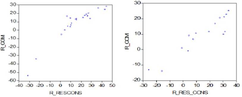
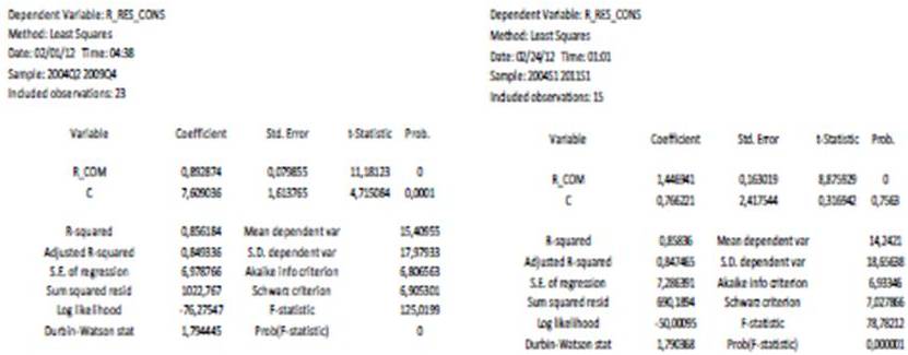
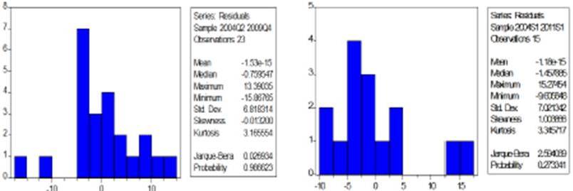
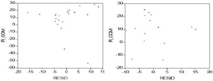
The Parameters Estimations and the Econometric Model’s Tests

The correlation between the two variables of the model is described by the following graphics:

Fig. 1 Return on Used Resources Vs. Return on Sales for Petrom (left) and Zentiva (right)

After applying the OLS method for estimating the model’s parameters, the equations become:

Petrom: Return on used resources (R_RES_CONS) = 7,60 + 0,89 * return on sales (R_COM)

Zentiva: Return on used resources (R_RES_CONS) = 0,76 + 1,44 * return on sales (R_COM)

Fig. 2 The Parameters Estimations for the Econometric Model Using the OLS Method for Petrom (left) and Zentiva (right)

The value of the coefficient “b” shows that for an increase of the return on sales, the return on used resources enhances with 0,89 (Petrom) and with 1,44 (Zentiva). In other words, this coefficient indicates that the objective variable, the return on used resources, increases with 0,89 (Petrom) or with 1,44 (Zentiva) when the return on sales increases with one unit. The causal relationship between the objective and the independent variable is a direct one because the value of the coefficient “b” is positive.

The coefficient “a” indicates the level of the return on used resources independently of the return on sales’ values, when the independent variable, the one that explains the cause of a certain level of the return on used resources, is zero.

From a graphic point of view, “b” means the imaginary line’s inclination that passes through the middle of the points from the scattering diagram of the return on used resources and the return on sales (fig. 1).

For the statistical implications of the estimations’ results previously shown (fig. 2) it was used a test called T student. Applying this test, it can be verified every parameter of the equations presented earlier:

Null Hypothesis: H0: a = 0

Alternative Hypothesis: H1: a â‰ 0
→ t statistic>t table and prob (t-stat) <5%→ the null hypothesis is denied

And

Null Hypothesis: H0: b = 0

Alternative Hypothesis: H1: b â‰ 0
→ t statistic>t table and prob (t-stat) <5%→ the null hypothesis is denied

Petrom (fig. 2): t statistic for the coefficient “a” (4,71) > t table for the coefficient “a” (2,080);

t statistic for the coefficient “b” (11,18) > t table for the coefficient “b” (2,080);

Zentiva (fig. 2): t statistic for the coefficient “a” (0,31) < t table for the coefficient “a” (2,160);

t statistic for the coefficient “b” (8,87) > t table for the coefficient “b” (2,160).

As a conclusion, for both companies, for the coefficient “b” the null hypothesis is denied: the coefficient “b” of the model is significantly dissimilar with zero. For the coefficient “a”, for Petrom, the null hypothesis is denied, but for Zentiva, the null hypothesis is accepted. Considering these aspects, the return on sales is a determinant factor of the return on used resources for both companies, but for Petrom one can confirm that, due to the fact that the null hypothesis for the coefficient “a” is also denied, choosing the return on sales as a determinant factor is correct.

In the following paragraphs, for the purpose of validating the econometric model, there are some defined aspects:

a) Îµi: N(0, Ïƒ2) (the errors are normally distributed);

b) Cov (Îµi, xi) = 0 (the errors are not correlated with the values of xi);

c) Var (Îµi) = Ïƒ2 (the variance of the errors is equal, homoscedasticity);

d) Cov (Îµi, Îµj) = 0, for i â‰ j (the errors are independent);

where, Îµi is the residual variable, errors,

xi is the independent variable.

For the accomplishment of the objective that refers to the normal distribution of the errors, I propose the following hypothesis and the normality or Jarque Bera test:

Null Hypothesis: H0: Îµi follow the normal distribution N (0,1);
Alternative Hypothesis: H1: Îµi do not follow the normal distribution N (0,1).

Fig. 3 Jarque Bera Test for the Model of the Return on Used Resources vs. the Return on Sales for Petrom (left) and Zentiva (right)

The results of the test for Petrom show that the value of Kurtosis is 3,16 and the value of Skewness is -0,01. One can conclude that if Kurtosis is of almost 3 and Skewness is around zero, the conditions of asymmetry and flattening are accomplished as for the residuals to be normally distributed. For Zentiva, Kurtosis (3,34) and Skewness (1,00) could signify that the errors distribution tends to be normal, but Skewness is not very close to zero.

As a rule, considering that the residual variable is normally distributed, Jarque Bera indicator asymptotically follows the chi-square distribution with 2 df. The Jarque Bera indicator for Petrom (0,02) is close to the value of 0,0201 (probability of 0,99), which means that there are sufficient reasons to accept the null hypothesis. For Zentiva, the Jarque Bera indicator (2,59) is close to the distribution of 2,408 (probability 0,30), which allows to be concluded that the null hypothesis is most probably denied.
Considering the above results, one can certainly say that the null hypothesis is accepted for Petrom and the residuals are normally distributed, and for Zentiva, the null hypothesis is denied.

For testing the correlation of the errors with the independent variable and for verifying if the errors variance is equal (homoscedasticity) or, with other words, for testing the assumption that the residuals are independent related to the evolution of each factor of the model, the following hypothesis can be formulated. These assumptions will be tested using graphics and using the White test. For the White test, the followingequation should be formulated: Îµi2= Î£ uj * xji + Î£ vj * xji2.
Null Hypothesis: H0: Cov (Îµi, xi) = 0, the errors are not correlated with the values of the independent variable;
Alternative Hypothesis: H1: Cov (Îµi, xi) â‰ 0, the errors are correlated with the values of the independent variable;

And

Null Hypothesis: H0: u1=…=uk=v1=…=vk=0, the errors are of constant variance (homoscedasticity hypothesis);
Alternative Hypothesis: H1: there is uj â‰ 0 or vi â‰ 0, the errors are not of constant variance (heteroscedasticity hypothesis);

The below graphics are for illustrating the relationship between the residuals and the independent variable for the two companies

Fig. 4 The Graphics for the Correlation between the Residuals and the Return on Sales for Petrom (left) and Zentiva (right)

Concluding, for both companies (fig. 4), the null hypothesis is accepted, that is the errors are not correlated with the values of the independent variable.

The White test is:

Fig. 5 The White Test for the Model of the Return on Used Resources vs. the Return on Sales for Petrom (left) and Zentiva (right)

Considering the above test, the value of Obs*R-squared (4,63) for Petrom is lower than the value of the chi-square distribution with 2 df and probability 0,05 (5,991) and in this case the null hypothesis is accepted, that is the homoscedasticity of the errors. For Zentiva, the value of Obs*R-squared (2,07) is also lower than the value of the chi-square distribution with 2 df and probability 0,05 (5,991) and the null hypothesis is accepted, that is the homoscedasticity of the errors.

For testing the objective of autocorrelation of the residuals, there are formulated two hypotheses and it is used the Durbin — Watson test:

Null Hypothesis: H0: the errors are not correlated;
Alternative Hypothesis: H1: the errors are correlated.

Fig. 6 The Graphics of the Residuals for Petrom (left) and Zentiva (right)

For Petrom, the value of the Durbin Watson indicator is 1,79 (fig. 2). In this case, the value is around 2 and the errors are not correlated due to the fact that the null hypothesis is accepted. For Zentiva, the indicator is also 1,79 which means that the null hypothesis is accepted and the errors are not correlated.

For augmenting the testing procedures of the proposed model, it is necessary to analyze the model’s reliability by using the R2 (R squared) indicator. For both companies, the indicator is of 0,85 which means that the power of explanation of the independent variable (the return on sales) over the dependent variable (the return on used resources) is high enough.

The Interpretation of the Results

The model’s parameters must be significantly different from zero and the T student test offers assurance with regards to the signification of the independent variable influence over the objective variable. The ideal situation is for Petrom, where the “a” and the “b” coefficients are significantly dissimilar with zero, according to the tests.

The Jarque Bera indicator follows the null hypothesis of the normal distribution of the errors for Petrom. The normal distribution has a great importance because, in case of a denial of the null hypothesis, one can argue that the t statistic value follows the T student distribution. For increasing the chances of the null hypothesis to be accepted, it can be used the method of enhancing the number of observations which could bring the normal distribution. The fact that for Zentiva, the null hypothesis is denied implies that there is a possibility of the data sample to be too small.

The model’s estimators could lose their precisions if as of the White test the null hypothesis of homoscedasticity is denied. However, for the model proposed, the null hypothesis is accepted for both companies.

Considering the Durbin Watson test, non correlation of the residuals is confirmed for both companies. This aspect shows that there is no error of specification such as the omission of an important independent variable.

Aspects Regarding the Model Validation, the Results, the Limits and the Future Proposals

The model which best meets the requirements of the statistical tests is for Petrom and that means there is a strong relationship between the return on used resources and the return on sales. The model can be validated and this is also confirmed by the R2 indicator which has the value of 0,85. These conclusions might have an explanation in the fact that the data sample is large enough for Petrom (23 observations) compared to Zentiva (only 15 observations).

Thus, the difference between the two companies refers to the number of observations that were taken into account and this fact could be the cause of the differences between the results as regards to the statistical tests. For Zentiva, except for Jarque Bera test and for the “a” coefficient that is not significantly dissimilar with zero, all the other tests follow the requirements. For amending the Jarque Bera indicator and for presenting good results in accordance with the null hypothesis, the solution of increasing the number of observations is not a feasible one due to the fact that there is no sufficient available information on the internet site for the periods before 2004 and after 2011. The solution of choosing quarterly observations for increasing the data sample for Zentiva cannot be taken into account for the same reason of lacking available information. It can be concluded that the model is fully validated for Petrom and for Zentiva this could be validated, but with some reservations and with the recommendation of model improvement by adding new observations for future analysis that start from these conclusions.

The specific literature on this theme does not include sufficient studies for evaluating the relationship between the return on used resources and the return on sales. This is why the results of this study bring some clear evidences of the correlation between the two rates. It is also true that the operational income and the operational result include the net turnover, and the net result has as a component the operational result, while between the operational result and the operational expenses there is a correlation. However, the econometric model which refers to the relationship between the two return rates comes to validate the proposed hypothesis and to contribute to the enrichment of the specific literature in this particular area.

Conclusions

This study aims to obtain a conclusion regarding the relationship between two return rates: the return on used resources and the return on sales for two companies that were selected based on several predetermined criteria. The results of this analyze refer to the validation of the relationship between the two rates.
In the specific literature, there is a common procedure to discuss about the performance of the companies using measurement instruments like return rates and the relationships between the rates are often analyzed. In their study, Check et al. (2009) conclude that there is a direct relationship between the return on assets and the return on equity rates (Check et al., 2009).

Furthermore, the results found by Changqi et al. (2010), in their study, show that the pre-merger performances of Chinese acquiring companies are positively correlated with the cross-border post-merger performances (Changqi et al., 2010). Like some other researchers have shown, the increased performance of the acquiring companies implies the presence of a very good management, efficient policies, which all have positive results on post-merger performances (Changqi et al., 2010). In this scenario presented by Changqi et al. (2010), measuring the performance means using the return on assets indicator. Once again, the instrument for measuring the performance is a return rate.

It can be concluded that the specific literature shows some evidences regarding the return rates as performance measurement instruments and regarding the existing relationships between them. However, as far as I know, there have not been put into discussion rates like the return on used resources or the return on sales, even though, a company may like to know if there is a relationship between the rates, in general or in their specific case. This is why the study is of high interest for the researchers from the specific area and for other parties.

The limits of this study are given by using only two companies and of a relatively reduced data sample, aspects that leave no room for generalized interpretations over a certain industry, country or over an entire category of companies. Although the two companies differ one from each other (have operational activities in two different areas and have different sizes), these also present similarities: for both companies the return on used resources is directly correlated with the return on sales (however some limits arise for the case of Zentiva).

Although, the results of this study cannot be generalized over other companies, they are useful, first of all, for Petrom and Zentiva managements. The managers of the companies could target their strategies considering the results of this study. Secondly, these results are useful for third parties interested in the evolution of the economic and financial performances of the two companies and for future scientific research studies from this area. This analysis is also useful for the elaboration of guides and books which have the topic of companies’ economic and financial performances and also in various debates and scientific conferences.

This study can be improved or can be a basis for future analysis related to this specific topic. I recommend to be taken into account as a larger data sample (at least 35 observations) and to consider annual data. Furthermore, one can choose another return on used resources calculation method, in order to obtain more accurate results.

Acknowledgements

This article is a result of the project „Doctoral Program and PhD Students in the education research and innovation triangle”. This project is co funded by European Social Fund through The Sectoral Operational Program for Human Resources Development 2007-2013, coordinated by The Bucharest Academy of Economic Studies.

References

Changqi, W. & Ningling, X. (2010). “Determinants of Cross-Border Merger & Acquisition Performance of Chinese Enterprises,” Procedia Social and Behavioral Sciences, 2, 6896—6905.
Publisher – Google Scholar

Check, H. F., Walker, J. S. & Randall Ka. L. (2009). ‘A Binary Choice Model for Predicting Bank Acquisitions,’ Journal of the Northeastern Association of Business, Economics and Technology, 15(1), 41 — 55.

Hagendorff, J. & Keasey, K. (2009). “Post-Merger Strategy and Performance: Evidence from the US and European Banking Industries,” Accounting and Finance, 49, 725—751.
Publisher – Google Scholar

Papadakis, V. M. & Thanos, I. C. (2010). “Measuring the Performance of Acquisitions: An Empirical Investigation Using Multiple Criteria,” British Journal of Management, 21, 859—873.
Publisher – Google Scholar

Petrom, www.petrom.com, 2012.
Publisher

Shim, J. (2011). “Mergers & Acquisitions, Diversification and Performance in the U.S. Property-Liability Insurance Industry,” Journal of Financial Services Research, 39, 119—144.
Publisher – Google Scholar

Vâlceanu, G., Robu, V. & Georgescu, N. (2004). ‘Analiză economico-financiară,’ Editura Economică, Bucharest, Romania.
Google Scholar

Zentiva, www.zentiva.ro. 2011.
Publisher

The Relationship between Two Return Rates as a Basis for Performance Evaluation

Journal of Economics Studies and Research

Claudia Maria Bulugea

The Academy of Economic Studies, Bucharest, Romania

Copyright © 2012 Claudia Maria Bulugea. This is an open access article distributed under the Creative Commons Attribution License unported 3.0, which permits unrestricted use, distribution, and reproduction in any medium, provided that original work is properly cited.

Abstract

The Relationship between Two Return Rates as a Basis for Performance Evaluation

Claudia Maria Bulugea

The Academy of Economic Studies, Bucharest, Romania

Copyright © 2012 Claudia Maria Bulugea. This is an open access article distributed under the Creative Commons Attribution License unported 3.0, which permits unrestricted use, distribution, and reproduction in any medium, provided that original work is properly cited.

Abstract

+Articles

+General Information