Introduction
Indonesia’s economic reforms began in the mid 1980s, when government made a monetary and fiscal deregulation in 1983. Over the next decade, reforms were expected at opening the real economy by promoting direct investment flows and liberalizing the financial sector, increasing competition, and promoting growth.
The government aimed to support these reforms with improved macroeconomic management, including through an attempt to maintain a competitive and stable exchange rate. The exchange rate policy was first changed in December 1978 from a pegged regime to a managed floating exchange rate system. The rupiah was linked to a basket of currencies consisting of Indonesia’s main trading partners.
The crude petroleum and natural gas dominated the Indonesia’s export trade until the mid 1980s. Hence, the oil price largely influenced and determined the government‘s earnings. The collapse of oil price in 1986 led to a devaluation, and government was pushed to boost non-oil/gas exports.
After the two major devaluations in 1983 and 1986, Bank Indonesia strived to intervene against the foreign exchange market in order to stabilize the exchange rate, country’s foreign exchange reserves and monetary system.
When the financial crises occurred in 1997, rupiah depreciated and continued to slide and exceeded the upper limit of the intervention band. Bank Indonesia decided to float the rupiah on August 14, 1997. Indonesia was the worst sufferer in the Asian crisis. The nominal exchange rate jumped from Rp2400 per US dollar to almost Rp17000 per US dollar in mid 1998.
This paper attempts to analyze and test the monetary approach and the overshooting hypothesis in Indonesia. It emphasizes the effect of financial liberalization to the exchange rate of Indonesia in the period of before and after the economic crisis. The model of exchange rate determination is expressed as a function of the relative money supply, relative income level, the nominal interest differential and the expected long-run inflation differential. We use the ordinary least square (OLS) method in the analysis and applying the Chow test in order to explore the stability of rupiah before and after the economic crisis.
Literature Review
As the fixed exchange rate system had terminated, many of the literatures began to explain the exchange rate changes. These literatures are laid on monetary or asset view. The older theories of exchange rate are focused more on trade of account of the balance of payments, while new theories; that are called “asset view,” focused on a stock approach.
Frankel (1979) suggests that there are two very different approaches in new theories. The first approach might be called the Chicago theory. It assumes that prices are perfectly flexible. If there is a change in nominal interest rate, it will reflect changes in the expected inflation rate. When the domestic interest rate rises relative to the foreign interest rate, there will be a decrease in home currency through inflation and depreciation. So there will be a positive relationship between the exchange rate and the nominal interest rate differential.
The second approach might be called the Keynesian theory. It assumes prices are sticky, at least in the short run. If there is a change in the nominal interest rate, it will reflect changes in the tightness of monetary policy. When the domestic interest rate rises relative to the foreign rate, it will attract a capital inflow, which causes the home currency to appreciate. So there will be a negative relationship between exchange rate and the nominal interest differential.
The monetary approach to exchange rate determination focuses on the money market. The interaction between money demand and money supply results in an equilibrium exchange rate. Thus, the exchange rate is seen as the equilibrium price between two stocks of money.
In the monetary model, there are some assumptions applied. Firstly, the money supply is assumed to be stable and exogenous. Secondly, assets are perfectly substitutable; therefore, UIP (Uncovered Interest Parity) holds continuously. Thirdly, the demand for money is a stable function of fundamental variables such as income and interest rate. Fourthly, income is assumed to be at its full-employment level. Finally, PPP is assumed to hold continuously.
The exchange rate of a monetary model is determined by relative money demands and money supplies. If domestic income increases fairly to foreign income, then the demand of money for domestic will increase relatively to the supply. Consequently, this causes the exchange rate appreciates. By contrast, an increase in the domestic money supply causes to augment in the exchange rate. The excess supply of money results in depreciating the exchange rate respectively. Similarly, if expected domestic inflation rises about the expected in the foreign country, then the demand for money falls and the exchange rate will depreciate.
Dornbusch (1976) introduced his sticky-price monetary model, which contained an overshooting hypothesis. The main feature of his model is that since prices are sticky in the short-run, an increase in the money supply will result in lower interest rate and thus capital outflow, will cause currency depreciation. In the short run, the currency will overshoot itself. However, over time, commodity prices will rise and result in a decrease in real money supply and higher interest rate. In the end, the currency will appreciate.
The empirical researches about the exchange rate determinants are varied. The works of Frankel (1979), Driskill (1981), and Papel (1998) provide the overshooting model, while Backus (1981) and Flood and Taylor (1996) do not. Hairault et al. (2004) finds that an expansionary monetary policy implies an increase in interest rate and a depreciation of the exchange rate.
Obstfeld and Rogoff (2000) have recently underlined the difficulty in estimating the exchange rate volatility. Any models are underlying fundamentals such as interest rates, outputs and money supplies but no model seems to be very good at explaining exchange rates even ex-post.
Model
The theory of monetary approach begins with two fundamental assumptions. The first is the interest rate parity. The market is efficient which bonds of different countries are substitutable.
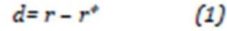
Where r is defined as the log of one plus the domestic rate of interest and r* is defined as the log of one plus the foreign rate of interest. If d is considered to be the forward discount, defined as the log of the forward rate minus the log of the current spot rate, subsequently equation (1) is a statement of covered (or closed) interest parity. However, d will be defined as the expected rate of depreciation; then equation (1) represents the stronger condition of uncovered interest rate parity.
The second is that the expected rate of depreciation is a function of the gap between the current spot and an equilibrium rate, and of the expected long-run inflation differential between the domestic and foreign countries:
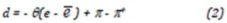
Where e is the log of the spot rate and and * are the expected inflation home and foreign country. The log of the equilibrium exchange rate Ä“ is defined to increase at the rate of – *. Equation (2) says that in the short run the exchange rate is expected to return to its equilibrium value at a rate which is proportional to the current gap, and in the long run when e = Ä“ , it is expected to change at the long-run rate – *. The rational value of will be seen to be closely to the speed of adjustment in the good market.
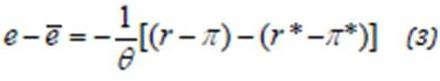
Combining equation (1) and (2) gives:
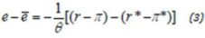
The equation in the bracket shows the real interest rate differential. When a tight monetary policy in one country causes the nominal interest differential to rise above its long-run level, an incipient capital inflow causes the value of the currency to rise proportionally above its equilibrium level.
Assuming that in the long run, purchasing power parity holds:
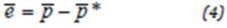
Where p and p* are defined as the logs of the equilibrium price level at home and foreign country.
Assume that the function of money demand equation:
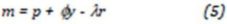
Where m, p and y are defined as the logs of the domestic money demand, price level and output. Assume also money demand equals to the money supply. A similar equation holds abroad, and the different between the two equations for home and foreign are:

Considering that in the long run, e = Ä“, á¹ = á¹*, – * , we get


This equation illustrates the exchange rate of monetary theory is determined by the relative supply of and demand for two currencies. The equation (8) shows that exchange rate will increase if rising in the domestic money supply, falling in income and increasing in inflation.
With Dornbusch-Frankel sticky-price monetary model and modified money demand function, this paper specifies the fundamentals for nominal exchange rate determination model:

where  (*) denotes a variable of the foreign country, s is the logarithm of the spot exchange rate (rupiah per US$), m is the logarithm of the money supply (M2), y is the logarithm of real income, r is the short-term interest rate, rate, π is the expected inflation rate, and μ is the disturbance term. Indeed, monetarist would predict the estimate of y = 1, while in overshooting hypothesis, y > 1.
Methodology
This paper uses the ordinary least square method in order to see the factors that influence the exchange rate of Indonesia. Some tests have been set up to give the best estimation. Before estimating the regression, the data will be tested to make sure that the data is valid and reliable, by using such as the normality test, linearity test, and stationarity.
After that, this paper implements a co-integration technique to detect whether a stable long-run relationship between exchange rates and fundamental variables exists. Co-integration methodology allows researchers to test for the presence of equilibrium relationships between economic variables.
Prior to testing for co-integration, we need to examine the time-series properties of the variables. They should be integrated of the same order to be co-integrated. In other words, variables should be stationary after differencing each time series the equivalent number of times. Therefore, at the first step, we develop unit root test to find the non-stationary level.
Unit Root Test
Ganger and Newbold (1974) suggested that in the presence of non-stationary variables, there might be a spurious regression. A spurious regression has a high R2 and t-statistics that appear to be significant, but the results are without any economic meaning.
The time series of m, y, r, and π are in fact non-stationary time series, that is generated by random process and can be written as follow:

Where εt is the stochastic error term that follows the classical assumptions, which means, it has zero mean, constant variance and is non-auto correlated (such an error term is also known as the white-noise error term) and Z is the time series. Since we need to use the stationary time series for the next co-integration test, and we also need to solve this unit root problem, therefore, we will run the regression of unit root test based on the following equation:

Where we add the lagged difference terms of dependent variable Z to the right-hand side of equation (2). This augmented specification is then used to test:
Ho: b= 0 H1: b < 0
Therefore, both the Augmented Dickey-Fuller (ADF) and Phillips-Perron (PP) statistics are used to test the unit root as the null hypothesis.
Co-integration Test
Engle and Granger suggested that co-integration refer to variables that are integrated of the same order. If two variables are integrated of different orders, they cannot be co-integrated.
Under the unit root test, the results show that the variables of exchange rate, money supply, output, interest rate and inflation are stationary at the first difference [I(1)]. Continuously, all the variables will be tested in co-integration test, by using the Johansen test statistics, imply that if exchange rate and macroeconomic fundamental are co-integrated, so there is a long term equilibrium relationship between these variables.
At the end of the analysis, we use Chow Breakpoint Test in order to check the stability of rupiah after government implemented the free floating exchange rate in the third quarter of 1998.
The Data Set and Test Results
The data used in this paper aimed to test the relationship between the exchange rate of rupiah per U.S. dollar and the Indonesia and U.S. fundamental macroeconomic variables. The sample of this research is quarterly data taken from International Financial Statistics from 1997 until 2004. The study employed the quarterly market exchange rate to measure the exchange rate. To measure income, we used the three-monthly Gross Domestic Product. The quarterly M2 was used to measure money supply. Then the three-month deposit rate was used to compute the interest rate variable. Last not but least, to measure the CPI variable was a quarterly consumer price index. All of data is expressed in logarithm except the interest rate.
Stationarity Test
The estimated regression will be more precisely if using stationary data. In order to check the stationary data, this paper uses the unit root test.
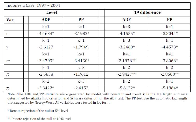
Table 1: Augmented Dickey-Fuller (ADF) and Phillip-Perron (PP) Statistics for Exchange Rate and Macroeconomic Fundamental
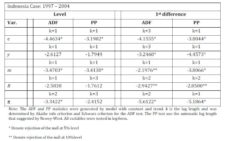
Table 1 presents the results of both unit root tests for the exchange rate of rupiah per US dollar and measure of fundamental macroeconomic variables for Indonesia and United States in levels and first difference. The ADF test fails to reject the null hypothesis at the 5% level for some variables such as output (y) and interest rate (r). Similarly, the PP test also fails to reject the null hypothesis for the same variables.
However, the ADF and PP test rejected the null hypothesis for all variables in the first difference at 5% level, except the variable of interest rate (r), which is at 10% level. Since all variables are stationary at first difference, therefore, it is an I(1) stochastic process. The finding implies that it is reasonable to proceed with test for co-integrating relationship between combinations of these series.
Estimated Regression
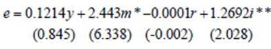
To predict the factors influencing exchange rate determination of Indonesia, then the regression is built using OLS method. The result using the data 1997.3 until 2004.1 is as follows:
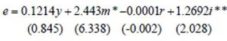
R2 = 0.748 F = 16.366 DW = 2.136
* Denote rejection of the null at 5% level
** Denote rejection of the null at 10%level
The data of variable y, m, r and i are domestic minus foreign data. The result shows that the signs of variables are the same as the hypothesis, except output. The sign of this variable should be negative; however, this data is insignificant. The other variable that is insignificant is interest rate, but it has the right sign. The implication of this finding is the interest rate is not a proper instrument in order to influence the exchange rate. When the central bank of Indonesia increases the interest rate will only make the exchange rate appreciate a little bit, and it is insignificant.
Money supply and price are significant in influencing the exchange rate of Indonesia. The increase of money supply and interest rate makes the exchange rate depreciate. An increase 1.0 percent of the money supply in Indonesia will depreciate between rupiah to 2.4 percent. This means rupiah is very sensitive to the money supply. The implication of this finding is the central bank has to control the exchange rate in order to stabilize the rupiah.
The results reveal that the elasticity obtained for relative money supply m is greater than unity (2.443). It indicates that one-percent increase in Indonesia’s relative money supply will cause a long-run depreciation of the rupiah by 2.443%, a result consistent with overshooting hypothesis.
Price is also significant influencing the exchange rate. Indonesia’s inflation in 1998 has been worsening the exchange rate. An increase 1.0 percent of inflation will stimulate depreciation of rupiah about 1.2 percent.
The Structural Change of Indonesia Currency
When involving time-series data, it might trigger the structural change. If the structural change happens, the values of the parameters of the model do not remain the same through the period due to external forces. The crisis hits Indonesia may also cause the structural change of Indonesia’s exchange rate. This paper uses Chow Test in order to see the stability of Rupiah after government changed the exchange rate system from the managed floating exchange rate to free floating exchange rate in 1998. The result of Chow test is as follows:
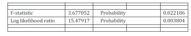
Table 2: The Result of Chow Test
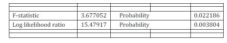
The Chow test result shows that F values in the estimated model does exceed the critical F value at =5%. We can also check to its p value which is lower than level of significant, and that means there is a structural change of rupiah before and after Indonesia choosing the free floating exchange rate system. The implication of this finding is rupiah is instable before and after economic crisis.
Co-Integration
This paper implements a co-integration technique to detect whether a stable long-run relationship between exchange rates and fundamental variables exists. Co-integration methodology allows researchers to test for the presence of equilibrium relationships between economic variables.
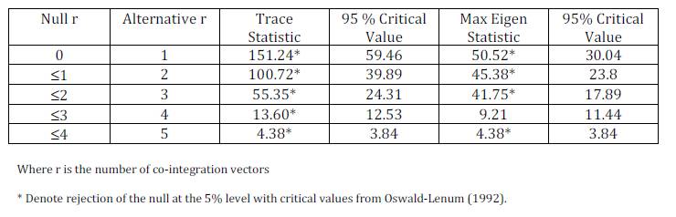
Table 3: Co-Integration Results (With a Linear Trend)
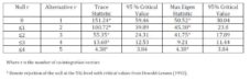
The parameter estimates of the co-integrating model are reported in Table 2. The Johansen test rejects the null hypothesis at 5% which proves the existence of co-integrating relationship among exchange rate, output, money, interest rate and inflation. Therefore, this result indicates five co-integrating equations at 5% significant level using Trace Statistic. However, based on Max Eigen Statistic there are three co-integrating equations.
Conclusion
This paper examines the nature of linkages between exchange rate and macroeconomic fundamentals. It also attempts to find out whether rupiah is stable or not after financial liberalization in 1998 when the government implemented the free floating exchange rate system.
We conduct several econometrics tests in order to establish the appropriate estimated regression. We also test the stationarity of each time series in order to estimate the co-integrating relationship in the long run and short run. The findings have identified that all time series are stationary at the first difference in the Augmented Dickey-Fuller and Phillip-Perron test. Consequently, the Johansen co-integrating test shows that the exchange rate and macroeconomic fundamentals are co-integrated in the long run. The latter, we use Chow test to prove that rupiah is instable after the financial liberalization. The finding shows that there is a structural change in rupiah.
Overall, the paper’s finding suggests that money and interest rate influence exchange rate significant either in short-run or long-run. Therefore, the monetary institution of Indonesia should be aware of these two variables in order to stabilize the exchange rate, moreover, the economic performance. The elasticity obtained for relative money supply m is greater than unity indicating that this result consistent with overshooting hypothesis.
References
Backus, D. (1984). “Empirical Models of the Exchange Rate: Separating the Wheat from the Chaff,” Canadian Journal of Economics, 17, 824—846.
Publisher – Google Scholar
Bahmani-Oskooee, M. (1998). “Do Exchange Rates Follow a Random Walk Process in Middle Eastern Countries?,”Economics Letters 58, 339—344.
Publisher – Google Scholar
Bahmani-Oskooee, M. & Kara, O. (2000). “Exchange Rate Overshooting in Turkey,” Economics Letters, 68, 89—93
Publisher – Google Scholar
Dornbusch, R. (1976). “Expectations and Exchange Rate Dynamics,” Journal of Political Economy, 84, 1161—1176.
Publisher – Google Scholar
Driskill, R. A. (1981). “Exchange Rate Dynamics: An Empirical Investigation,” Journal of Political Economy, 89, 357—371.
Publisher – Google Scholar
Flood, R. P. & Taylor, M. P. (1996). “Exchange Rate Economics: What is Wrong with the Conventional Macro Approach?,” In: Frankel, J.A., Galli, G., Giovannini, A. (Eds.), Micro Structure of Foreign Exchange Markets, The University of Chicago Press.
Publisher – Google Scholar
Frankel, J. A. (1979). “On the Mark: A Theory of Floating Exchange Rate Based on Real Interest Differentials,” American Economic Review, 69, 610—627.
Publisher – Google Scholar
Hairault, J. O., Patureau, L. & Sopraseuth, T. (2004). “Overshooting and the Exchange Rate Disconnect Puzzle: A Reappraisal,” Journal of International Money and Finance, 23, 615—643
Publisher – Google Scholar
Kim, S. & Roubini, N. (2000). “Exchange Rate Anomalies in the Industrial Countries: A Solution with a Structural VAR Approach,” Journal of Monetary Economics, 45, 561—586.
Publisher – Google Scholar
MacDonald, R. & Taylor, M. P. (1993). “The Monetary Approach to the Exchange Rate,” IMF Stafff Papers, 40, 89—107.
Publisher – Google Scholar – British Library Direct
Obstfeld, M. & Rogoff, K. (2000). “The Six Major Puzzles in International Macroeconomics: Is there a Common Cause?,” In: Bernanke, B., Rogoff, K. (Eds.), N.B.E.R Macroeconomic Annual 2000. MIT Press, Cambridge, MA, 339—390.
Publisher – Google Scholar – British Library Direct
Papel, D. H. (1988). “Expectations and Exchange Rate Dynamics after a Decade of Floating,” Journal of International Economics, 25, 303—317.
Publisher – Google Scholar