Introduction
It is well established that over extended time horizons, leveraged ETF’s returns often diverge significantly from the product of their daily leverage ratio and their periodic benchmark return. This is due to the nature of the daily rebalancing and constant leverage these funds maintain. Explicitly, this return drift is defined as the leveraged ETF’s return over a given time period minus the leverage ratio of the ETF multiplied by the underlying index return. While this return drift may be positive or negative, investors are primarily concerned with negative drift, which this study refers to as decay. The primary cause of this decay is the volatility of the underlying index; the greater the volatility, the faster and more severe the decay, (Cheng and Madhavan, 2009; Trainor, 2009).
However, Trainor (2011) points out that the limited holding periods that have been suggested for these funds are not a foregone conclusion. If volatility levels are sufficiently low, positive compounding caused by directional market moves in favor of the fund can actually outweigh the negative volatility effect.
Thus, for investors choosing to hold leveraged ETFs for extended periods of time, positive outcomes rely not only on making a correct market call in terms of its direction, but also on the magnitude of the underlying index volatility that will be experienced. Although leveraged funds will never be long-term buy and hold investments, in many market environments leveraged funds can be successfully held for extended periods without experiencing significant decay.
The oversight in the literature is not quantifying how long investors may want to consider holding these funds given a particular index return forecast. To answer this question, this study quantifies the decay-volatility tradeoff and derives optimal holding periods given an investor’s decay threshold under various volatility environments. Since volatility is known to be persistent, reasonable forecasts for how long leveraged funds can be held before experiencing significant decay relative to their daily leverage ratio can be made. Thus, an investor who holds a 3.0x leveraged ETF and expects the underlying index to increase 3% over the next 3 months, can evaluate whether a 3-month holding period in the leveraged ETF is justified. For example, if the expected decay is -2%, the investor is taking on 3x the risk for 2.3x times the expected return, (3.0 x 3.0% – 2.0% decay).
This study develops a theoretical model to measure decay relative to leverage, volatility, return trend, and time. Using a GARCH (1, 1) model to forecast volatility, maximum decay estimates are shown to be rarely exceeded for holding periods out to 3 months. Using a decay threshold of -2%, a level which will obviously be unique to each investor, theoretical holding periods are derived for a myriad of leverage ratios and volatility levels. The use of the model is empirically demonstrated for leveraged ETF stock funds over the last 8 years.
The remainder of this paper is organized as follows. A short history and literature review is given which is followed by a theoretical model to measure return drift where decay is a special case. A demonstration of this model shows the relationship between decay, leverage, volatility, return trend, and time. The next section uses a GARCH (1, 1) model to predict volatility which allows the drift model to be empirically applied to equity data over the last 8 years. The paper concludes with a brief summary.
Literature Review
Leveraged index mutual funds have been available since 1993, and the first leveraged ETF was introduced by Proshares in the summer of 2006. Currently, there are more than 200 ETFs with approximately $40 billion in assets providing daily leverage from -3.0x to 3.0x on indexes covering everything from stocks to coffee. Investors quickly realized that the unique property of constant daily leverage led to long-term holding period multiples that lag the daily multiple. This return “decay” resulted in some long (short) leveraged funds to actually be down even when the underlying index was up (down). Theoretically, given a high enough volatility, almost any long-term multiple is possible with the most likely scenario being a deterioration in the long-term multiple. Both the popular press and academic studies have made substantial note of this fact and generally suggest very short holding periods for leveraged funds, (Trainor & Baryla, 2008; Carver, 2009; Avellaneda & Zhang, 2010; Lu, Wang, & Zhang, 2009; Justice, 2009; Lauricella, 2009; Spence, 2009, 2010; Zwieg, 2009; Maxey, 2009).
Theoretical models developed to model the relationship between leveraged ETFs and the underlying index generally assume that the underlying index return follows a standard Ito process, (Cheng and Madhavan, 2009; Avellaneda & Zhang, 2010). These studies demonstrate why volatility is such a critical factor in determining the long-term leverage ratio of a constant fixed leveraged fund. Empirically, studies have found that the deterioration of the long-term multiple is almost certain.
However, this result is certainly skewed by the fact that most leveraged ETFs were introduced right before the financial crisis when volatility levels spiked. In September 2009, Direxion actually changed their daily leveraged mutual funds to monthly leveraged funds to at least partially address the decay issue associated with daily funds. However, Trainor (2010) found that after 6-months, the difference in the deterioration of the long-term multiple between a daily and monthly rebalanced leveraged fund becomes fairly blurred. The critical factor is volatility. Trainor (2011) shows that if leveraged funds had existed during more mundane volatility periods, that a leveraged ETF return drift can actually be positive with leverage ratios enhanced as opposed to being reduced. A study by Deng, McCann, and Wang (2012) suggest hedging leveraged ETFs to reduced volatility appears to allow enhanced realized leveraged ratios.
Based on the literature, a rationale for extended holding periods can be made depending on the return drift, which in general, is usually negative and referred to in this study as decay. This study directly identifies the length of holding periods that can be maintained given an investor’s particular decay threshold. This information is crucial to an investor who has an expected return for the underlying index over a particular period of time, and wants to know the expected return/risk tradeoff when using leveraged ETFs to enhance this return.
Drift-Decay Model
By their design, daily leveraged ETFs magnify the underlying index on a day-to-day basis only. Over time, the actual return to a leveraged ETF can virtually be any multiple relative to the underlying index return. In volatile markets, the offsetting return moves will cause a leveraged ETF to a have a long-run multiple less than the daily multiple. This is what is referred to as decay. To formally derive this concept, consider the 2 period case. The underlying index return (XR) over two periods is:
(1) XRT = [(1+r1)(1+r2) -1] = r1 + r2 + r1r2
And the return to a leveraged fund (LRT) is:
(2) LRT = [(1+βr1)(1+βr2) -1] = βr1 + βr2 + β2 r1r2
Where β is the leverage point. After two periods, if β remains constant through time, equation (2) should equal βr1 +βr2 + βr1r2. Thus, the difference between LRT and XRT relative to a time constant beta is:
(3) LRT – βXRT = (β2 – β)*r1r2 (2 PERIOD CASE)
As an example, if the index is up 10% then down 5%, Equation (1) shows that the two period return should be 4.5% and Equation (2) shows that a 2x would only be up 8.0% instead of 9.0%, for a realized two period leverage ratio of 1.78. Equation (3) simply relates the difference, which in this case is -1.0%. This is the decay.
More generally, for any time period T, the difference between a leveraged fund and the index return relative to a time constant beta involves the cross terms of a Tth dimensional multiplicative matrix minus the squared terms of the diagonals. This gives us:
(4) 
Where ε is the product of higher order terms. Since  =
=  then
then 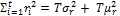 where µr is the mean of ri and is the standard population variance. Substitute and using summation rules, we have:
(5) 
For Large T, we can simplify and approximate to:
(6)  (N period Case).
Equation (6) shows the relationship between decay and  for any µr. It is easy to see the competing effects of the mean and standard deviation. The greater the magnitude of the return over a particular time period, the smaller the decay. In fact, if the return over a particular time period is large enough, the actual leverage experienced can be greater than the daily leverage ratio. Equation (6) also clearly shows the negative effect of higher levels of volatility. One may also note how bearish leveraged funds experience greater decay relative to bullish funds for any absolute level of leverage by examining the (β2 – β)/2 term in equation (6). For example, (β2 – β)/2 for a -2x is 3 and for a 2x it is only 2.
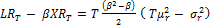
Furthermore, by taking the first derivative of equation (6) with respect to µr, the maximum decay for any T can be shown to occur when µr = 0:
(7) 
Equation (7) reaches zero at any of the following conditions: µr = 0, T = 0, β = 0, or β =1. The economic interpretation of this minimum for T and β is straightforward. At T=0, the market has yet to move, and hence there is no decay. At β=0, there is no investment and there is no potential for decay, and at β=1, the ETF is unlevered. At μr=0 the market’s average return is zero. We can see that the critical point μr=0 is in fact a minimum by noting that the second derivative of equation (6) is T2(β2-β). Now, T2 is positive everywhere, and β2-β >0 for all β outside of the interval [0, 1]. As a result we observe that for any given volatility level, the maximum possible decay occurs when the market return is zero. This is an important result since the absolute maximum decay an investor will experience for any particular leverage over any time frame is not dependent on predicting the return of the market, but only on predicting the volatility that will be experienced.
Model Application
Given historical market returns and standard deviations, equation (6) proves continuous decay is to be expected. Inputting an annualized mean and standard deviation of 10% and 20% respectively, a 2x fund can expect to be down 3 percentage points in a year relative to two times the underlying index return. A 3x fund can expect to be down 9 percentage points within a year. This is the basis for most studies concluding that investors should not hold these funds for any extended period of time.
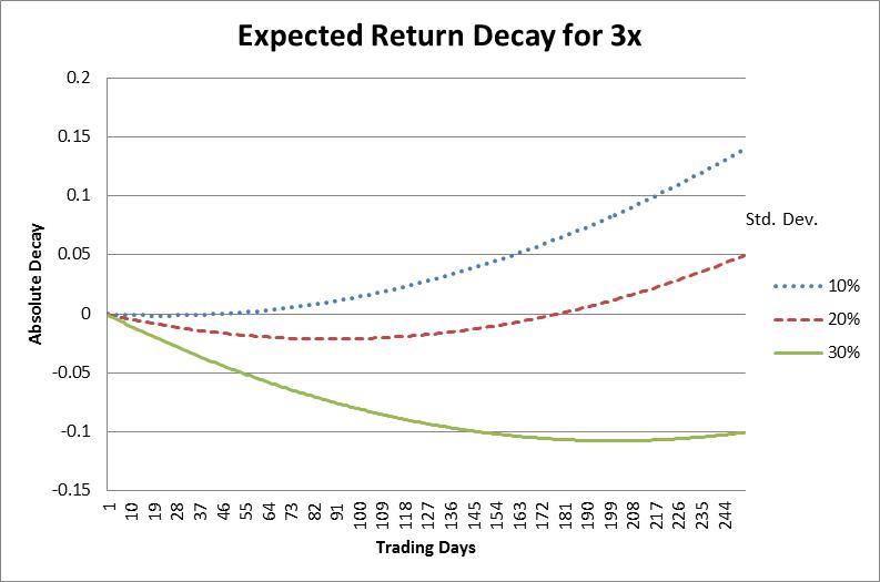
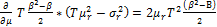
However, this long-run leverage deterioration is not preordained. To demonstrate this, Figure 1 shows the decay for a 3x leveraged fund under the assumption of a 2% non-annualized monthly return and annualized standard deviations ranging from 10% to 30%. Although the 30% standard deviation environment still shows the 3x fund return will decay relative to 3 times the underlying index return, lower levels of volatility show that the 3x fund will actually attain more than the daily leverage would imply. In essence, the positive trend outweighs the negative volatility effect. It should also be noted here that the realized leverage will never be larger than the daily leverage when the underlying index moves against the fund.
Figure 1: Theoretical Decay for a 3x Fund Assuming a 2% Monthly Return
Given an investor is willing to accept a certain amount of decay, equation (6) can also be used to indirectly calculate a maximum holding period that an investor should consider. By setting µr in equation (6) equal to 0, the maximum decay for any time T can be derived. This implies a maximum holding period that an investor would want to consider based on the investor’s decay threshold, assuming the underlying volatility environment remains relatively unchanged. Figure 2 graphically displays this given a -2% decay threshold across the volatility spectrum.
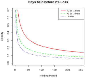
Figure 2: Length of Holding Period Before -2% Decay is Reached
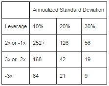
Numerically, Table 1 summarizes the holding periods for leveraged funds given 10%, 20%, and 30% volatility levels with a -2% decay threshold assuming μr = 0. With volatility levels fairly low, decay is rather mitigated with holding periods for the -1x or 2x beyond a year. For the 3x and -2x funds, holding periods out to 8 months can be justified. Obviously the investor still needs to make the correct market call, but losses will be limited to which direction the market moves, and not a significant function of volatility. Any trend, regardless of direction, will reduce the negative impact of decay and may even push the decay term to net positive if the trend is strong enough to the benefit of the fund. In general, low volatility extends the time prior to decay thresholds being reached resulting in the situation where investment returns will be primarily determined by market direction.
Table 1: Maximum Holding Periods in Trading Days before Decay Falls to More than -2%.
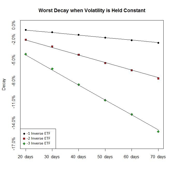
Although the above results are based solely on equation (6), the theoretical decay derivation is quite accurate. Using both actual and simulated data for all leverage ratios and time frames out to one year, the actual decay and theoretical calculated decay values are virtually identical. Figure 3 below illustrates this accuracy. We note that at μr = 0 equation (6) reduces to a linear function of time when volatility is held constant. By holding volatility constant at 30%, Figure 3 overlays the worst observed decay for a given time period on top of the linear function predicted by equation (6). The data used in this simulation was the Russell 2000 over the period of 12/31/1979 through 8/31/2011.
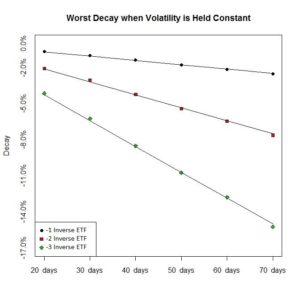 Figure 3: Worst Decay for a Given Volatility Level and Holding Period
However, the inputs used in equation (6) are the actual ex post mean and standard deviation realized over each particular time period examined. This only shows the model is correct when the inputs are actually realized. Since forecasting returns over any time T is virtually impossible, forecasting the actual decay that will be realized over any time T is also impossible. However, it was shown earlier that the maximum decay for any time period T will occur when the mean return over that time period is zero. Thus, the only critical input becomes the volatility over the time period T. Due to the persistence of volatility, this can be forecasted with some reliability and thus, a forecasted maximum decay can be relatively accurate.
Using GARCH to Forecast Holding Periods
The maximum holding period model’s utility will increase with the accuracy of volatility forecasts. Fortunately, volatility is known to maintain long periods of stability. Relative to ex post returns, ex post volatility realizations are not subject to the same magnitude of forecast error. For example, a 10% mean coupled with a 20% standard deviation only allows an investor to forecast the mean with a 95% confidence in any given year to within 40 percentage points of 10%. In contrast, based on Monte Carlo simulation, the actual standard deviation will be within 1.7% of the forecasted 20% volatility estimate in any given year.
In practice, the above narrow band will not necessarily hold due to structural changes in the market. Schwert (1989) shows that market volatility is related to general economic variables such as inflation and industrial production. Consumer confidence is also likely involved. Thus, the underlying standard deviation may not remain at 20%. Fortunately, there is a great deal of empirical evidence that shows volatility is relatively persistent for a period of time before switching regimes.
The study of volatility persistence has its roots in Mandelbrot (1963) and it is often modeled using an AutoRegressive Conditional Heteroskedastic (ACRH) process (Engle, 1982), or the Generalized ARCH (GARCH) process of Bollerslev (1986). It also has been shown to have two fairly significant properties: 1) periods of high volatility are associated with declining stock prices and 2) when volatility is high (low) it tends to remain high (low). Kritzman (2010) recently finds the same qualitative properties using a turbulence measure and suggests market volatility is more likely to erupt as financial assets become more integrated.
To give an idea of the significance of property 1 listed above, Table 2 shows the returns for the Center for Research Security Prices Value Weighted Index (similar to the Wilshire 5000) when market volatility is above its average and when it is below average. The results over the last 20 years have changed little relative to the last 80+. During low volatility months, the average monthly return has been 1.64%. During high volatility months, it has averaged -0.2%. Annualized, this is the difference between 21.5% and – 2.3% a year. Some studies have suggested that one can take advantage of this “volatility anomaly” by investing in low volatility stocks no matter what the overall volatility outlook is, (Ang, et. al, 2006, 2009).
Table 2: Historical Monthly Returns When Volatility is below and above Average.

The repercussions of Property 1 for leveraged funds is obvious. In application, any significant increase in volatility is going to be a double edged sword for bullish investors as both the expected decay would increase, and based on historical precedence, stock prices would be expected to fall as well. For the bearish leveraged fund investor, the tradeoff of the expected decline in stock prices due to an increase in volatility must be tempered by the higher decay rate. Historically, higher volatility dominates suggesting holding periods should be decreased.
As for Property 2, the persistence of volatility is fairly well established and this study employs a standard GARCH (1,1) to model persistence. This models the variance at time t as a function of a constant, the t-1 squared log return, and the t-1 variance. Mathematically, it can be written as:
(8) 
The greater α + β is in Equation (8), the greater volatility persistence is.
To empirically apply and test this model, the parameters are estimated for the Russell 1000 index from January 1993 to December 2002 and then used to make predictions through May 2011. It is interesting to note that these estimated parameters change very little when using the whole time period and are almost identical to the parameters estimated using the CRSP index as well.
The solutions using maximum likelihood estimation for the 1993 to 2003 time period shown in Table 3 are:
Table 3: Parameter Solutions for Equation (8) Using Maximum Likelihood Estimation.
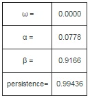
As one can see, the persistence is extremely high suggesting volatility tends to remain at whatever its current level is. As a practical matter, using this to forecast volatility is relatively straightforward. Given the calculated parameters, an estimate for volatility for any time T into the future is:
(9) 
Figure 4 shows the actual annualized rolling 3-month standard deviation and forecasted standard deviation ending at each time T. As one can see, the GARCH (1,1) model follows actual volatility fairly closely. It is only during the 2008 crisis when volatility levels change dramatically that the GARCH (1,1) forecasts lag significantly.
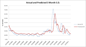
Figure 4: Actual versus Forecasted Decay for Rolling 3-Month Holding Periods from 2003 to May 2011
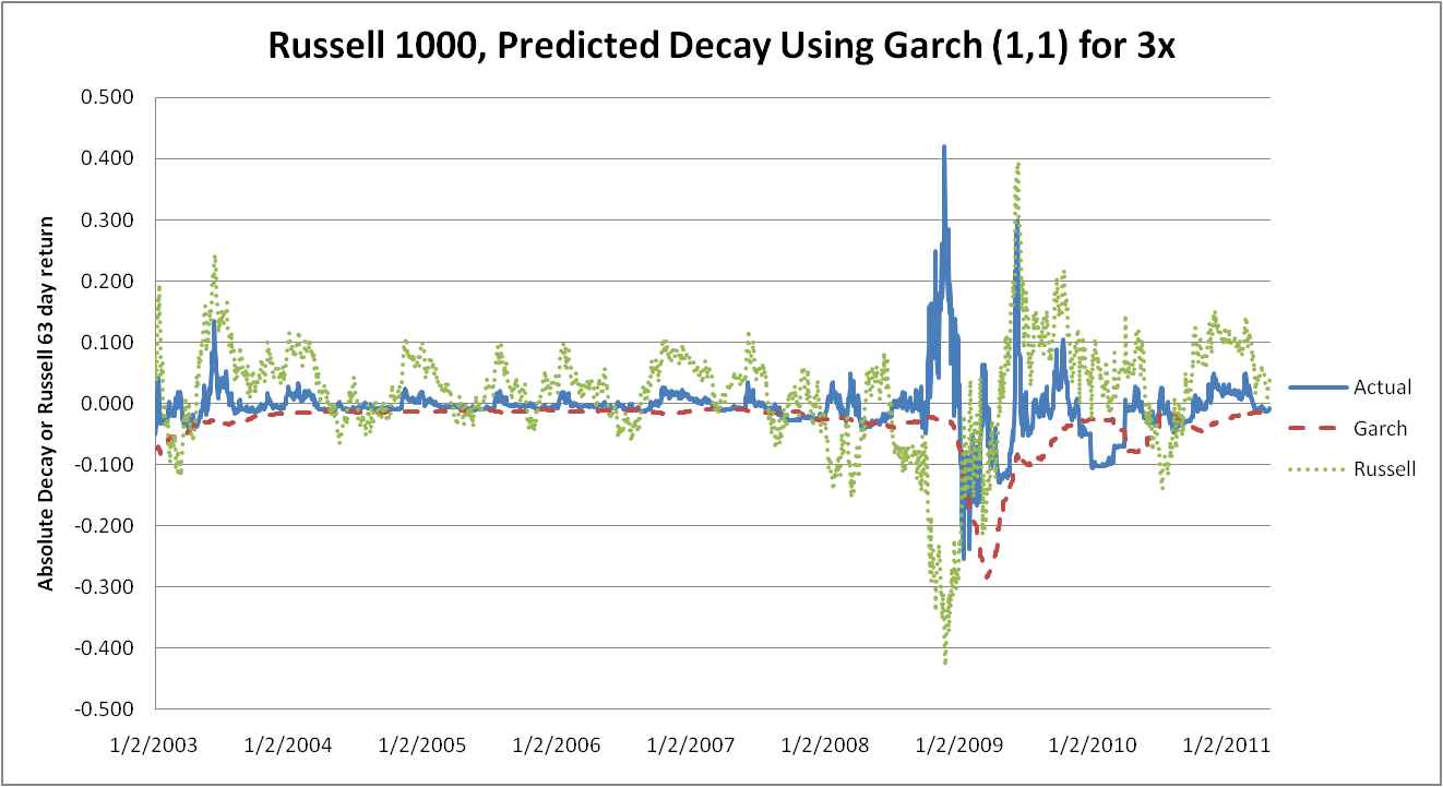
Once the GARCH (1, 1) volatility forecasts are estimated, these values are inputted in equation (6) to forecast decay. Figures 5 and 6 show the predicted maximum decay for a 3x and -3x respectively along with the non-annualized Russell 1000 63-trading day return. As long as volatility is relatively stable, the model rarely underestimates absolute decay. The only time this error will be significant is if the forecasted volatility vastly underestimates the realized volatility. This occurs during the turbulent 2008 financial crisis. It is more often the case that the forecasted absolute decay is much greater than the actual decay. This can be seen throughout the last 10 years and occurs whenever the return over the 3-month period moves significantly in the same direction as the fund’s leverage, or the volatility falls to much less than excepted.
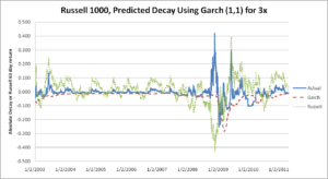
Figure 5: 3x Actual vs. Forecasted Decay for 3-Month Holding Periods
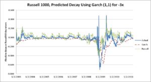
Figure 6: -3x Actual vs. Forecasted Decay for 3-Month Holding Periods
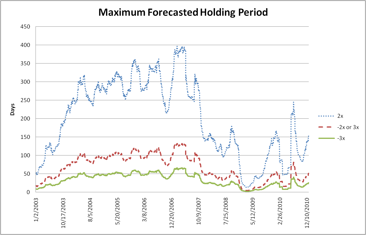
Using the -2% maximum decay threshold, Figure 7 shows the summarized implied maximum holding periods for leveraged funds from 2003 through 2010. Except for recent history, the average holding period in any given year, even for a 3x is usually more than 2 months.
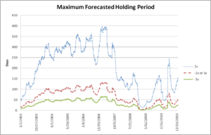
Figure 7: Forecasted Holding Periods Based on GARCH (1,1) 3-Month Volatility Forecasts
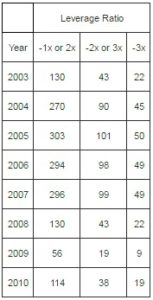
Table 4 numerically summarizes Figure 7 and shows the average maximum holding periods for the last 8 years. During the financial crisis, the implied holding period was only 19 days for a -2x or 3x. To the extent volatility levels return to their longer term averages, positive outcomes for longer holding periods will become more apparent given correct market calls by investors.
Table 4: Average Forecasted Maximum Holding Periods in Days.
Conclusion
Leveraged funds are not a long-term buy and hold investment. Based on market return and volatility averages, there is an inherent expected decay in leveraged ETF returns over time. However, this decay is not substantial in low volatility environments and can even be outweighed by significant trend.
The main question that has remained about these investments is exactly how long an investor can expect to hold these assets and not experience appreciable leverage deterioration relative to the return they might expect given the daily leverage ratio. This study answers that question by developing a model that calculates maximum decay for any leverage ratio over any time frame given return and volatility inputs.
When volatility levels are relatively low as they were in the 90’s and mid 2000’s, holding periods beyond a year for 2x and -1x funds can be justified. For 3x, -2x, and -3x funds, holding periods out to 6 months can be justified. When volatility levels are more “normal,” holding periods of 1 to 3 months for -2x, 2x and 3x funds are justified while high volatility levels suggest holding periods of 1 month or less. According to Guedj, Li, and McCann (2010), some investors are indeed holding the least popular funds for extended periods of time as they find more than 8% of investors in certain leveraged ETFs have holding periods of more than 3 months .
Using a maximum decay criteria which occurs when the market has a zero cumulative return, volatility forecasts from a GARCH (1, 1) model are used to forecast decay. For 3-month horizons, actual absolute decay rarely exceeds projected. Only during the 2008 financial crisis when volatility parameters were changing dramatically did actual decay significantly exceed projected. Due to volatility persistence, maximum holding periods for leveraged funds in which the return/risk tradeoff is not significantly compromised due to decay can be forecasted with some degree of confidence. When this occurs, investors can be relatively confident that if the market is up (down) 5% within a forecasted maximum holding period, that their 3x (-3x) fund will be up close to the 15% they are expecting.
As the reader may have noted, volatility forecast error, and thus decay forecast error only became pronounced to any significant degree during the financial crisis. The drastic increase in volatility caused the GARCH (1, 1) forecast to underestimate volatility and hence, expected decay. Thus, the accuracy of this model is limited to the degree volatility remains relevantly persistent. The model put forth in this study does not immediately adjust to dramatic shifts in volatility. Future research focusing on the refinement of the volatility forecast model could improve the results. Incorporation of the VIX and the use of more advanced GARCH models may be able to adjust to volatility regime changes more quickly.
The empirical testing of the model has also been limited to equities. Future research in applying the model to leveraged ETFs on commodities, foreign exchange, and interest rates are just a few avenues open to both researchers and investors. As long as the underlying instrument demonstrates relatively persistent volatility, the application of this model to estimate decay, and by extenuation, reasonable holding periods for investors should be functionally accurate. This will allow leveraged ETF investors to calculate the maximum decay over any time horizon to better gauge the risk/return tradeoff they face.
(adsbygoogle = window.adsbygoogle || []).push({});
References
Ang, A., Hodrick, R. J., Xing, Y. & Zhang, X. (2006). “The Cross-Section of Volatility and Expected Returns,” Journal of Finance, 61, pp. 259-299.
Publisher – Google Scholar
Ang, A., Hodrick, R. J., Xing, Y. & Zhang, X. (2009). “High Idiosyncratic Volatility and Low Returns: International and Further U.S. Evidence,” Journal of Financial Economics, 91, pp. 1-23.
Publisher – Google Scholar
Avellaneda, M. & Zhang, S. (2010). “Path-dependence of Leveraged ETF Returns,” Society for Industrial and Applied Mathematics, 1, pp. 586-603.
Publisher – Google Scholar
Bollerslev, T. (1986). “Generalized Autoregressive Conditional Heteroskedasticity,” Journal of Econometrics, 31, pp. 307-27.
Publisher – Google Scholar
Carver, A. B. (2009). “Do Leveraged and Inverse ETFs Converge to Zero?,” Institutional Investor Journals, ETFs and Indexing, 1, pp. 144-149.
Publisher – Google Scholar
Cheng, M. & Madhavan, A. (2009). “The Dynamics of Leveraged and Inverse Exchange-Traded Funds,” Journal of Investment Management, 7(4).
Publisher – Google Scholar
Deng, G., McCann, C. & Wang, O. (2012). Are VIX Futures ETPs Effective Hedges?, Working paper.
Publisher – Google Scholar
Engle, R. F. (1982). “Autoregressive Conditional Heteroskedasticity with Estimates of the Variance of United Kingdom Inflation,” Econometrica 50, pp. 987-1007.
Publisher – Google Scholar
Guedj, I., Li, G. & McCann, C. (2010). “Leveraged and Inverse ETFs, Holding Periods, and Investment Shortfalls,” The Journal of Index Investing, Vol.1, No. 3, pp. 45-57.
Publisher – Google Scholar
Justice, P. (2009). “Warning: Leveraged and Inverse ETFs Kill Portfolios,” Morningstar Investing Specialists. Available at http://news.morningstar.com/articlenet/article.aspx?id=271892, 22 January.
Publisher – Google Scholar
Kritzman, M. & Li, Y. (2010). “Skulls, Financial Turbulence, and Risk Management,” Financial Analysts Journal, Vol. 66, No. 5, pp. 30-41.
Publisher – Google Scholar
Lauricella, T. (2009). ‘ETF Math Lesson: Leverage Can Produce Unexpected Returns,’ Wall Street Journal, 4 January.
Google Scholar
Lu, L., Wang, J. & Zhang, G. (2009). “Long term performance of leveraged ETFs,” Available at SSRN: http://ssrn.com/abstract=1344133, 15 February.
Publisher
Mandelbrot, B. (1963). “The Variation of Certain Speculative Prices,” Journal of Business, 36, pp. 394-419.
Publisher – Google Scholar
Maxey, D. (2009). “ProShare Draws Suit Over a Leveraged ETF,” Wall Street Journal, 7 August.
Publisher
Schwert, G. W. (1989). “Why Does Stock Market Volatility Change Over Time,” Journal of Finance, pp. 1,115-1,153.
Publisher – Google Scholar
Spence, J. (2009). “Short Plays Only, Holding Leveraged and Inverse ETFs too Long Distorts Objectives,” Market Watch, Available at http://www.marketwatch.com/news/story/leveraged-inverse-etfs-short-termplays/story.aspx?guid=%7B7BD723A4%
2DC1C2%2D4302%2DBD49%2DEE8B8EBB3AA0%7D&dist=TNMostMailed, 18 January.
Publisher
Spence, J. (2010). “SEC Inspects Derivatives-Based Funds,” Market Watch, Available athttp://www.marketwatch.com/story/leveraged-etfs-under-sec-scrutiny-2010-04-11, 11 April.
Publisher
Trainor, W. J. (2009). “The Effect of Time, Trend, Volatility, and Leverage on Relative Returns,” Direxion Funds,accessed July 28, 2012, available at http://direxionshares.com/pdfs/DS_Paper_011210.pdf, pp. 1-29.
Publisher
Trainor, W. J. (2010). “Daily vs Monthly Rebalanced Leveraged Funds,” Journal of Finance and Accountancy, Vol. 6, 2010, pp. 1-14.
Publisher – Google Scholar
Trainor, W. J. (2011). “Solving the Leveraged ETF Compounding Problem,” Journal of Index Investing, Vol. 1, No. 4, pp. 66-74.
Publisher – Google Scholar
Trainor, W. J. & Baryla, E. A. (2008). ‘A Risky Double that Doesn’t Multiply by Two,’ Journal of Financial Planning, 21, pp. 48-55.
Google Scholar – British Library Direct
Zweig, J. (2009). ‘How Managing Risk with ETFs Can Backfire,’ Wall Street Journal, 27 February.
Google Scholar