Introduction
Researchers and policymakers have paid a considerable attention to investigate the linkage between stock prices and macroeconomic variables. Stock market has a pivotal role in the growth of the industry and commerce that eventually affects the economy of the country to a great extent.
The theoretical framework had explained the relationship between stock market and macroeconomic factors, through different models. Present Value Model (PVM) formulated by Smith (1925), Primary Discount Model later advanced to Gordon Growth Model (GGM) formulated by Gordon (1962), Capital Asset Pricing Model (CAPM) formulated by Sharpe (1964), Linter (1965) and Arbitrage Pricing Theory (APT) formulated by and Mosin (1973), Ross (1976).
Especially, APT provided an interpretation of the changes in the macroeconomic factors that may have affected stock prices. Generally, the above mentioned models explain the anticipated and unanticipated of any new information that is related to macroeconomic variables. Moreover, they might have an effect on stock prices from their impact on discount rate or the expected future dividends.
In addition, these models give an understanding of macroeconomic variables which are extremely valuable for policymakers and investors. As a result of the continuous pursuits by the individuals and institutions to achieve profits and mitigate the risk exposure, through the policies or macroeconomic condition changes. In general, investors are seeking to reduce the risk exposure in their investments. Thereby, policymakers require a precise comprehension of the relations between stock market and macroeconomic condition to formulate valuable policies which contribute to enhancing stock market development and economic growth, (Yartey, 2008).
The empirical studies that analyzed the development in stock markets indicated that markets have a crucial role to promote economic growth in emerging markets, (Kose et al, 2006; Deb and Mukherjee, 2008).
The Turkish stock market has unique features, it is like one of the leading emerging markets and it shows a different pattern of stock market movement either from developed countries or other emerging markets. Turkey’s stock market showed a remarkable growth in a number of listed companies, market capitalization and trading volume over a short period of time.
At the end of 2013, the number of listed companies has grown to 401 compared to317 in 2008. Market capitalization grew from $ 119 billion in 2008 to $ 308.7 billion in 2013. The annual trading volume increased from $ 261 billion in 2008 to $ 389.1 billion in 2013. After the crisis of 2001, the policymaker was given the opportunity to pay more attention on the microeconomic problem which fueled the crisis, following the macroeconomic instability.
Therefore, emerging stock markets have been identified as being at least partially segmented from global capital market. Hence, this study attempts to analyze the effect of macroeconomic variables that includes monetary policy instruments on the Turkish stock price index. It assumes that the selected variables may have effect on the share price index (TSPI) at both the short and long-run relationship. The macroeconomic variables are Index of Industrial production (IIP), Short-term interest rate (SINT), Money supply (M2), and Exchange rate (EXC), for the period span from January 2002 to December 2013.
The current study will contribute to the literatures that investigate the Turkish stock market in different ways. Firstly, the study analyses the period that witnessed a new monetary policy. Secondly, the study analysis the whole Turkish stock price index.
Thirdly, the study analyses the linkage between TSPI and macroeconomic variables via applying VAR frame work including the structure of break points as exogenous variables into the system, to overcome the effect of monetary policy changes. Finally, the study seeks to examine the disequilibrium period due to positive or negative shocks in order to determine the adjustment speed of Turkish stock market to reach its equilibrium.
Literature Review
This section investigates the empirical evidence on the diverse linkages that are found between macroeconomic factors and stock market in the literature. Broadly, the empirical evidence on the macroeconomic determinants of the stock market falls into two categories. One investigates the effect of macroeconomic factors on stock returns, while the other investigates the effect of macroeconomic factors on stock prices.
Examples of studies that examined the macroeconomic determinants of stock return are; Chen, et al. (1986), David, et al. (1989), Choi, et al. (1992), Groenwold, and Fraser. (1997), Lajeri, and Dermine (1999), Muradoglu, et al. (2001), Ewing, (2002), andMerikas, and Merika (2006).
Since this study falls in the second category, the following are reviews of the literature centered on the dynamic interaction between macroeconomic variables and stock price. For instance, Ibrahim and Hassan uddeen (2003) analyzed the dynamic linkage between stock prices and four macroeconomic variables; industrial production, money supply, consumer price index and exchange rate, for the period spans from Jan 1977 to 1998 in Malaysia.
The findings suggest the presence of long-run and short-run relationship between the three variables and the stock prices. Particularly, it documents positive short run and long run relationships between industrial production and consumer price index variables and the stock price. Also, the result indicates the disappearance of the immediate positive liquidity effects of the money supply shock and understandable interactions between the stock price and the exchange rate over time. Another study of Maysam et al. (2004) examined the long-run equilibrium relationships between selected macroeconomic variables and the Singapore stock market index (STI), the finance index, the property index, and the hotel index for the period of Jan 1989 to December 2001.
The findings concluded that the Singapore`s stock market and property index form cointegration relationship with changes in the short and long-run interest rate, industrial production, price levels, exchange rate and money supply. Erdem et al (2005) examined the volatility spillover from inflation, interest rate, exchange rate, money supply and industrial production to Istanbul Stock Exchange’s stock prices index.
The study analyzed the period span from January 1991 to January 2004. The findings revealed that there is significant unidirectional spillover from macroeconomic variables to stock prices indexes except for services index.
Also, the findings show that there is a positive volatility spillover from exchange rate to both ISE 100 and industrial indices. Adrangi and Chatrath (2007) empirically introduced the dynamic linkage between stock market and inflation rate and seasonally adjusted industrial production index as proxy for real economic activity. The result showed that there is long run association between stock prices, general price level and real economic activity. Further, the findings revealed that there is a negative relation between stock price and unexpected inflation.
Rahman and Uddin (2009) examined the dynamic linkage between all share price index and exchange rate, in three emerging markets of South Asia namely: Bangladesh, India and Pakistan. Covering the period spans from January 2003 to June 2008.
The findings revealed that there is no co integration relationship between price indices and exchange rate by using Johansen procedure. Rjoub (2012) examined the dynamic relationship between exchange rates, US stock price as a world market and Turkish stock price index, for the period span from August 2001 to August 2008. By applying Vector Auteregression (VAR) framework, the finding revealed that there is long run relationship between variables.
Granger causality test indicates that there is bidirectional relationship between exchange rates and stock price. Issahaku and Ustarz (2013) investigate the dynamic relationship between stock price in Ghana and a set of macroeconomic variables namely: exchange rate, money supply, inflation rate and foreign direct investment for the period span January 1995 to December 2010 on monthly base. Applying Vector Error Correction Model (VECM), the findings revealed the presence of long-run relationship between stock price and a set of macroeconomic variables; inflation rate, money supply and foreign direct investment.
Furthermore, there is short run association between stock price and macroeconomic variables, interest rate, inflation rate and money supply. Lekobane and Khaufelo (2014) examined the ability of the stock market as a vivid reflection of the real economic activity through macroeconomic variables in emerging markets, to explore the long-run equilibrium relationship between Botswana stock price and the selected macroeconomic variables.
Using VECM framework following Johansen’s cointegration technique for the period spans from 1998 to 2012 quarterly base. The results indicated a positive long-run equilibrium relationship between stock market price and short-term interest rate, real GDP, inflation rate and diamond index. Moreover, there is negative relationship between Botswana stock market price and money supply, long-term real interest rate, exchange rate and US government bond yield.
Joseph and Jakkapong (2014) empirically examined the long-run equilibrium relationship between the selected macroeconomic variables and Thailand stock exchange index (SETI) for the period span from Jan 1990 to Dec 2009. Johansen cointegration analysis revealed that significant and positive long-run equilibrium relationship existed between SETI and money supply. However, consumer price index and industrial production index showed negative relationship with SET index over long-run equilibrium. Furthermore, error correction term indicated that the macroeconomic variables are selected to contribute to converging the equilibrium in Thailand stock exchange.
Methodology and Empirical Results
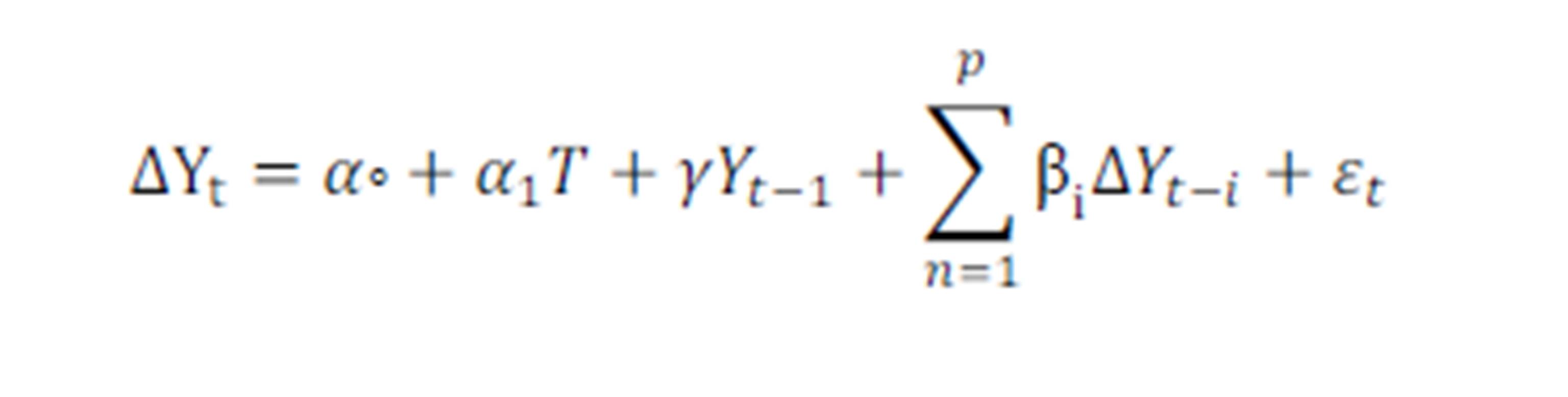
First of all, preliminary examination of the nature of the data series should be analyzed. The unit root tests were applied to investigate whether the data series of interest are stationary or not at level. For this purpose the study applies three types of unit root tests to generalize an idea about the nature of the series. The study follows the literature in testing the unit root by employing the Augmented Dickey Fuller ADF test in the general form:
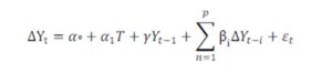
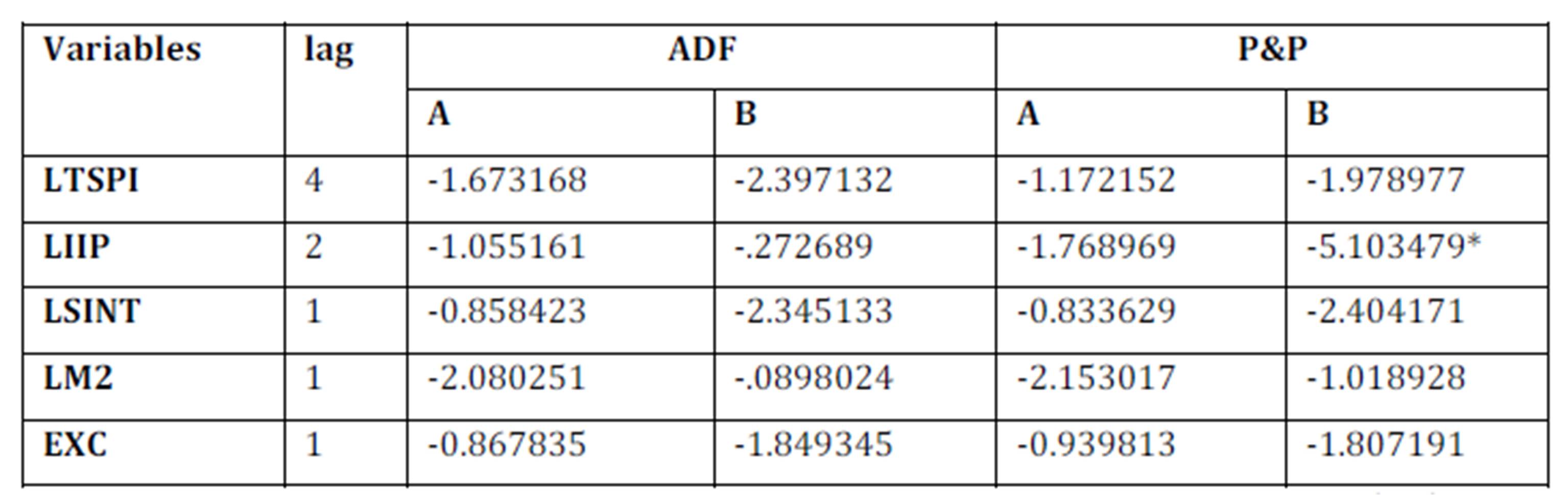
Where, Y represents the variables, and T are the differences and the time trend respectively. P represents the lagged value, represents the white noise residual. The study implements the Augmented Dicky Fuller (ADF) and Philip Perron (PP)tests with intercept, and intercept and trend. The form of PP unit root test is expressed as follows: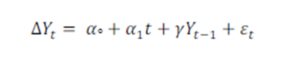 The variables and parameters are the same as the ADF unit root test in which they are defined. Null hypothesis of unit root tests of ADF and PP that mean the series has a unit root when γ = 0, that is against the alternative hypothesis of stationary, which implies that the time series is non-stationary. The results in Table 1 and Table 2 indicate that the variables have unit root at I (0), but they are stationary at I (1).
Table 1: Unit Root Test at the Level
*, **, and *** significant level at 1%, 5%, and 10% respectively, based on the test critical values. (A & B) with; intercept and intercept and trend respectively.
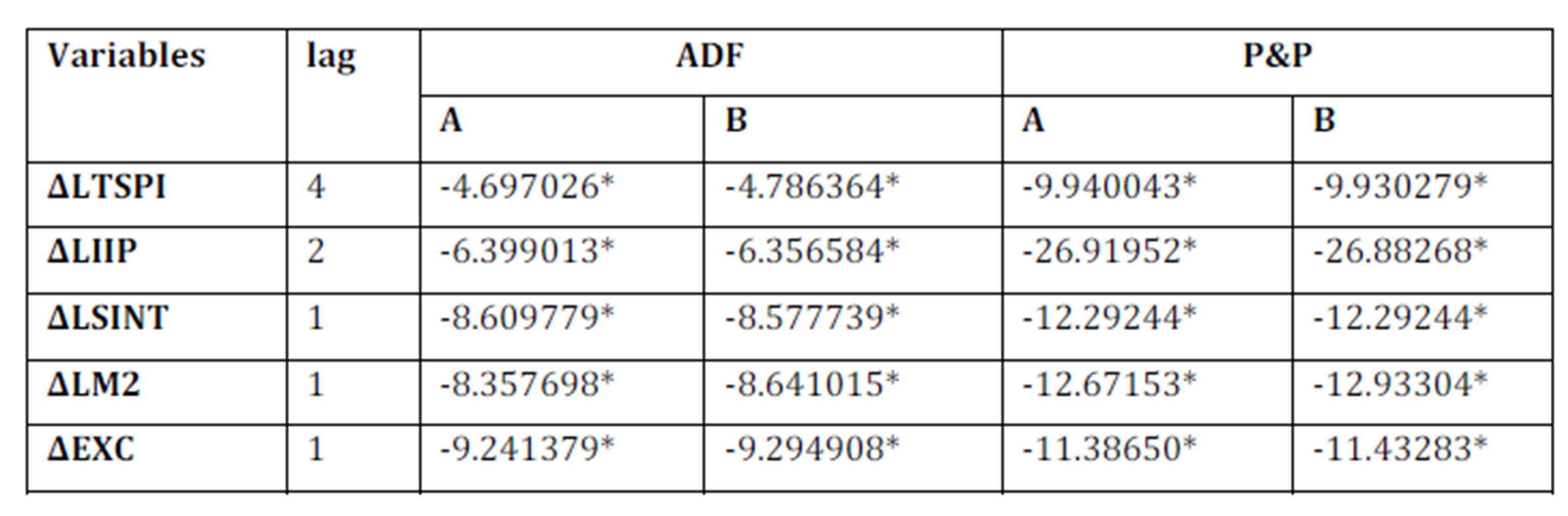
Table 2: Unit Root Test at the First Difference
*, **, and *** significant level at 1%, 5%, and 10% respectively, based on the test critical values. (A & B) with; intercept and intercept and trend respectively.
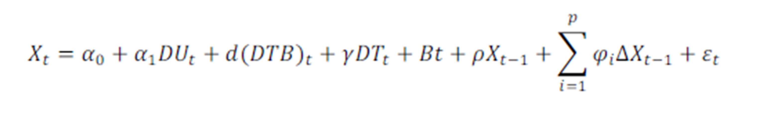
Most macroeconomic series are not distinguished by a unit root, but from the continuous infrequent and the large shocks. Thus, after the small and frequent shocks the economy comes back to deterministic trend. Hence, Zivot-Andrews (1992), unit root test with structural break verifying each possible break data using different dummy variables was expressed as follows:
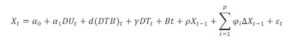
Where, dummy represents a change in the level =1 if (t>TB) and zero otherwise. The slope dummy represents the change in the slope of the trend function, dummy =1 if t=TB+1 and zero otherwise. TB represents the break data. This formula expresses the time series that have both intercept and trend.
Table 3: Zivot-Andrews (1992) Unit Root Test
*, **, and *** significant level at 1%, 5%, and 10% respectively rejecting the null hypothesis, has a unit root with a structural break in both the intercept and trend.
The results in Table 3indicate that the time series are stationary with structural break. Both LIIP and EXC are stationary with structural break due to domestic currency collapses. This means they may have been affected during the world crisis which took place in 2008.
Moreover, both LSINT and LM2 are stationary with structural break due to the changes in the monetary policy during the tested period. At the beginning of 2002, Central Bank of Republic of Turkey (CBRT) announced two nominal anchors: inflation target and monetary target mechanism to reduce “implicit inflation target”. The Short-term interest rate became the major policy tools of the monetary policy to lessen the inflation, (Civcir, 2009). Therefore, these studyaddeddummy variables for each factor into the VAR model according to the structure break point.
Many of the economic time series, such as consumption and income, stock prices and dividends have a theoretical long-run relationship.
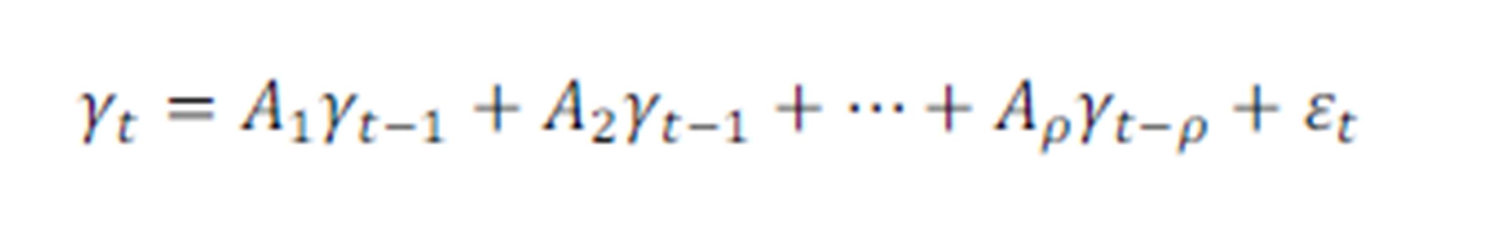
Also, it is generally accepted that these time-series data are changing over time, so their mean-value and variance are not constant (Nelson and Plosser, 1982). Based on these data, non-stationary time series, macroeconomists incorrectly conclude that two variables are related but in reality are not. Johansen cointegration test is a statistical method for testing cointegration based on a VAR model of order to examine long-run relationships that can exist between the variables.
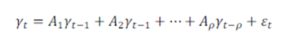
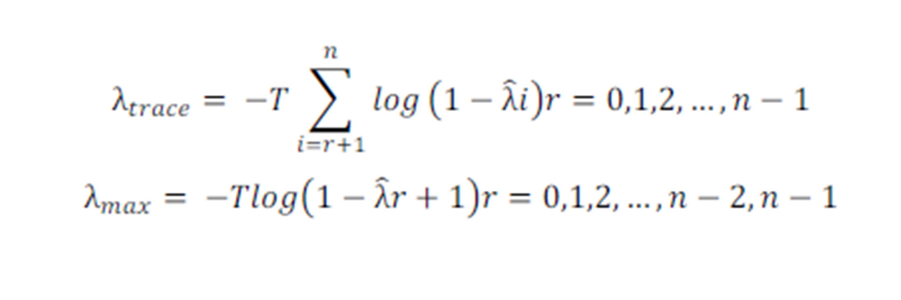
Where Ai`s are (NxN) coefficient matrices and is an unobservable i.i.d. zero mean independent white noise process at the lag five that indicates the absence of the serial autocorrelation. The optimal lag length determined based on Correlograms all the residuals are uncorrelated. That implies “white noise” residuals are estimated from the VAR system. The trace statistics and Max-eigen test statistics for the null hypothesis of cointegarting relation against the alternative of ncointegrating relations are computed as follow (Johansen, 1988):
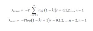
Where T is the number of observations and λ is the (i-th) largest eigenvalue. The maximum eigenvalue statistics test the null hypothesis of cointegrating relations Against the alternative of cointegrating relations.
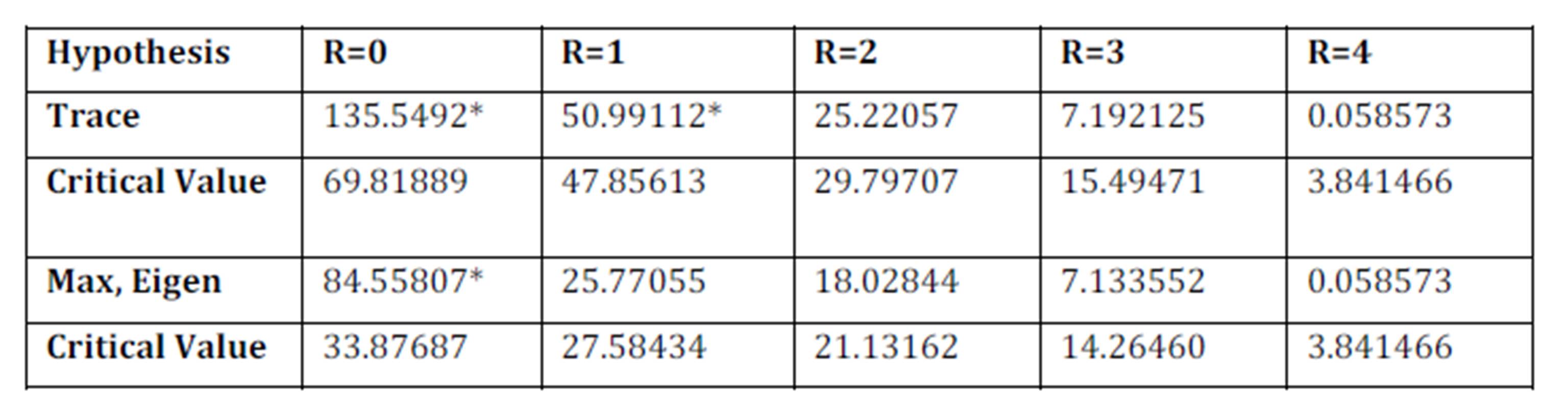
Table 4: Johansen Cointegration Test
*, rejecting the null hypothesis of no cointegration at 5% level. With optimal lag 5 white noise res
The findings in Table 4 reveal that there is long-run relationship between the LTSPI and the macroeconomic variables of interest. The cointegration equation isestimated as follows:
LTSPI = 3.961262 LIIP — 1.415689 LINT — 1.170528 LM2 — 0.559380 EXC
The results from long-run relation cointegration equation reveal that the variables have their anticipated signs. The finding reveals a positive relationship between Turkish stock prices and the industrial production index. Industrial production represents the real economic activity in Turkish economy, which indicates that it has direct influences on the firm’s future cash flow. The result is consistent with the empirical studies that investigated Turkish stock market, like Ahmad and Abdioglu (2010), and Cagli and Halas (2010). It is also consistent with the studies of Humpe and Macmillan (2009) for US and Japan stock markets.
The finding of the negative relationship between Turkish stock prices and the short-term interest rate implies that when the interest rate is high, the investors would not consider the Turkish stock market for their investment. After 2002, policymakers start to use the Short-term interest rate as a tool for monetary policy to fight the inflation rate. Thus, any increase in the real interest rate results in an increase in the risk and the required rate of return of the investments.
Therefore, increasing the cost of capital indicates the profits of a firm tend to decrease. The result is consistent with the findings of Buyuksalvarci (2010) and Zugul and Sahin (2009) that investigated the Turkish stock market. The same results were found to be identical withTeety (2008) for the Ghana stock market.
The negative relationship between TSPI and money supply (M2) was found. This is due to the changes in the monetary policy mechanism (restructuring period 2002-2007) to fight the inflation “inflation target” (where the inflation rate reached 35 percent for 2002 approximately).
This indicates that an increase in the money supply might result in an increase and generate inflation and might participate to inflation uncertainty. Hence, any increase in money supply might generate risk premium in turn leading equity prices to fall.
Thereby, exert a negative influence on Turkish stock prices. The findings are consistent with Zugul and Sahin (2009) that was conducted in Turkish stock market, as well as Ibrahim el al (2003) which was conducted on Malaysian stock market. Finally, the result reports a negative relationship between TSPI and EXC through the tested period.
This indicates an increase of the current and future cash flows of companies due to a depreciation of the domestic currency which would make local firms more competitive. Therefore, this is leading to an increase in their export and consequently higher stock price.
The negative long-run relation is consistent with empirical literatures conducted by Kasman (2003) and Rjoub (2012), both of which were conducted on Turkish stock market. The relation is also found to be consistent with the study of Raymond (2009) which was conducted on Jamaican stock market.
Concerning the dynamic analysis a principal feature of co integrated variables is that their paths are influenced by the extent of any deviation from long-run equilibrium. Therefore, if the system is to return to long-run equilibrium, hence there are at least some of the variables that must respond to the magnitude of the disequilibrium from their movements, (Enders, 2004; p328).
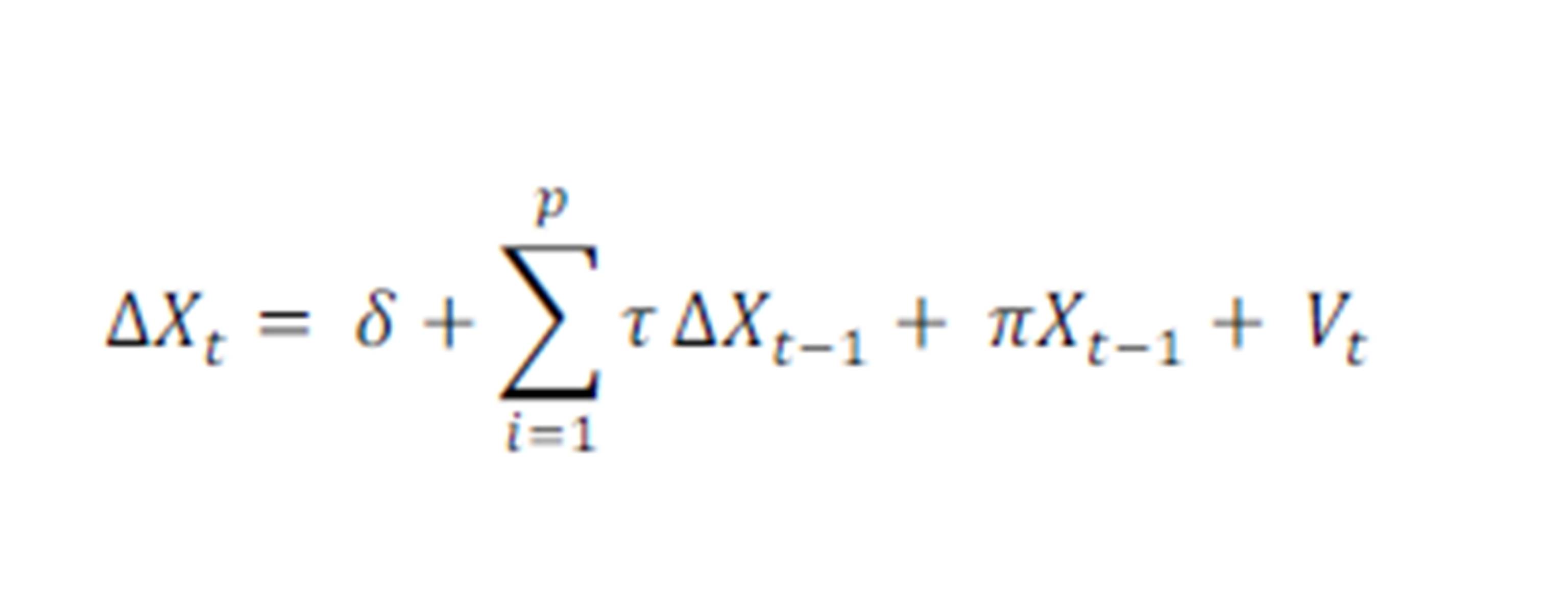
Adding the Error Correction Term (ECT) to capture the adjustment of the variables with respect to its long-run equilibrium, where the error term has no moving average part and the systematic dynamic, is kept as simple as possible. The variables are I(1) and they have a long-run relationship. There must be some forces that pull the equilibrium error back towards zero. The ECT does exactly this, to examine the behavior in the short-run which is consistent with a long-run co integration. ECT is expressed as follows:
Where;
ε ̂_(1t-1) And 〖ε̂〗_(2t-1) are the error correction term obtains from the long-run model.
〖∆X〗_(t-i) And〖∆Y〗_(t-1): Long-run values as predicted by the long-run model.
γ_1 And〖 γ〗_2: Capture the long-run causal relationship between the variables in the model.
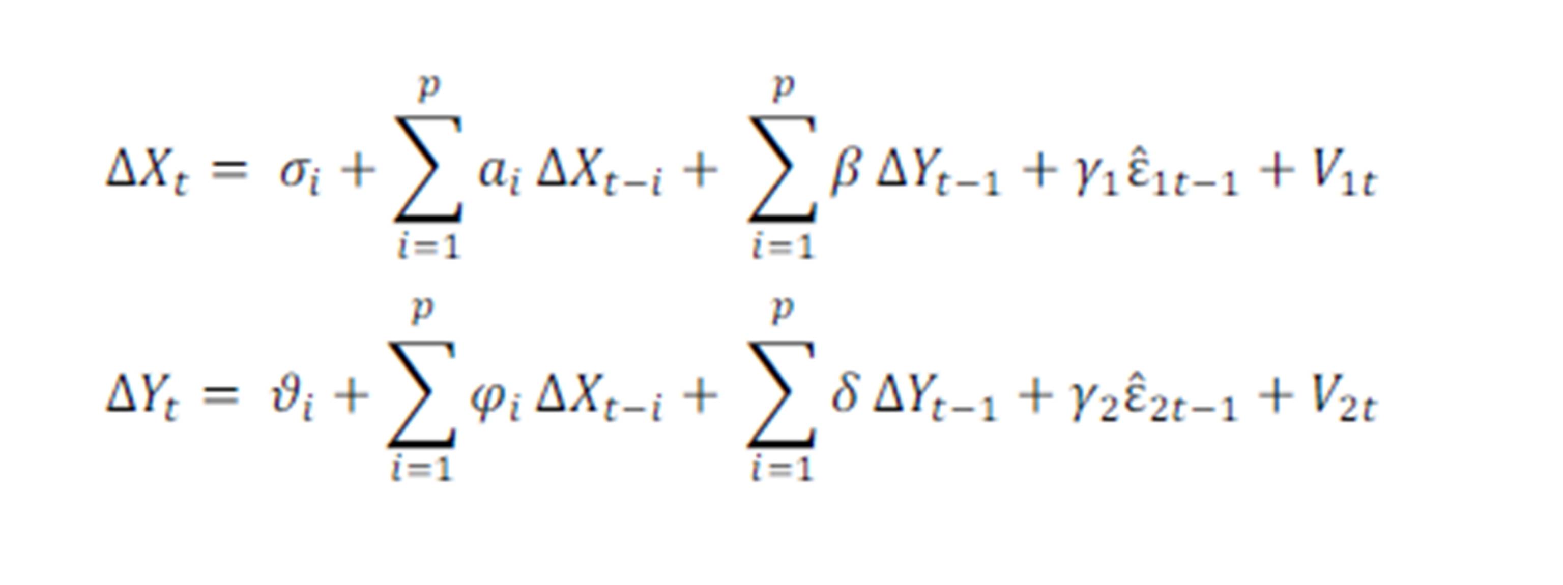
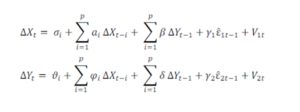
With the presence of cointegration relations, the VAR form is not the most convenient model setup. Thus, it is useful to consider specific parameterizations which support the analysis of the cointegration structure (Lütkephl, 2005). The result from subtracting γ_(t-1) from both sides and rearranging terms, a model known as Vector Error Correction Model (VECM) is found.Adding ECT into the model to investigate the short and long run dynamic adjustment of a system of cointegrated variables is expressed as follows:
Where;
〖∆X〗_t: is an (nx1) vector of variables.
δ: is an (nx1) vector of constant.
Ï€: Error correction term.
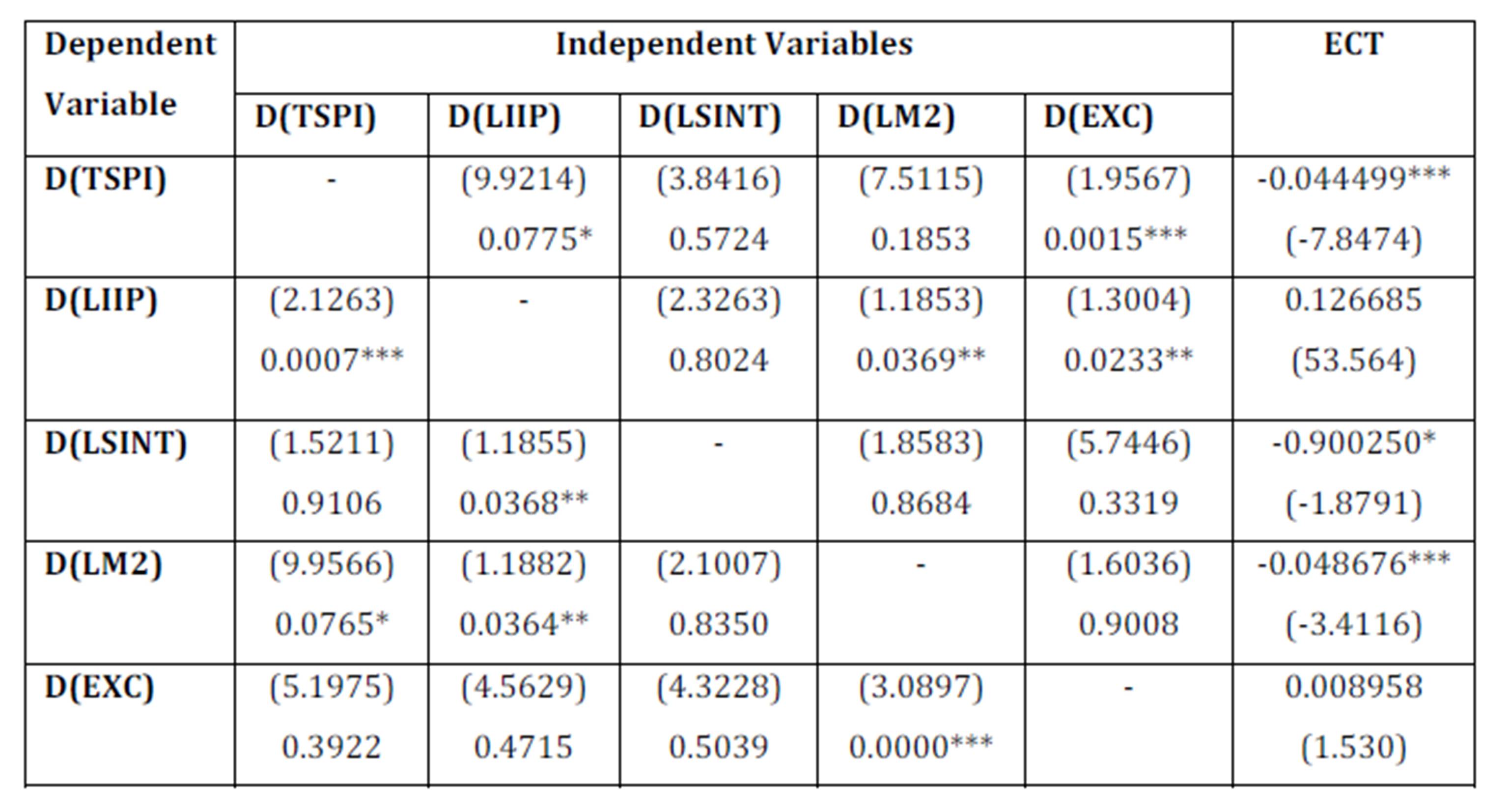
Table 5: VECM Causality Test Block Erogeneity Wald Test
***,**, *and significance level at 1%, 5%, and 10% respectively. The table contains both t-statistics associated with the error-correction term (ECT), The P-value isassociated with the x^2-statistic between parentheses; which represents the joint significance of the independent variable.
With the expected negative sign, the speed of adjustment (the coefficient) on the lagged ECT denoted a significant long-run causal effect given previously as results of Johansen cointegration. Moreover, the ECT indicates that Turkish stock market converges its equilibrium within 22.5 months after shocks. Thus, it is adjusting by 4.4499 % each month.
The results in table 5 reveal that EXC has unidirectional short-run granger cause on the LTSPI at 5% level of significance. The results are consistent with the findings of Erdem et al (2005) and Kasman (2003) for Turkish stock market, Issahaku and Ustarz (2013) for Ghana stock market.
The LTSPI has bidirectional granger cause with industrial production (LIIP),while it has a unidirectional on LM2. This indicates the LTSPI is considered as a leading indicator for two macroeconomic variables: LIIP and LM2. The findings are consistent with Ahmad and Abdioglu (2010) for Turkish stock market. They are also consistent with the study of Rymond (2009) for Jamaican stock market and Pilinkus (2009) for Lithuanian stock market.
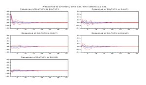
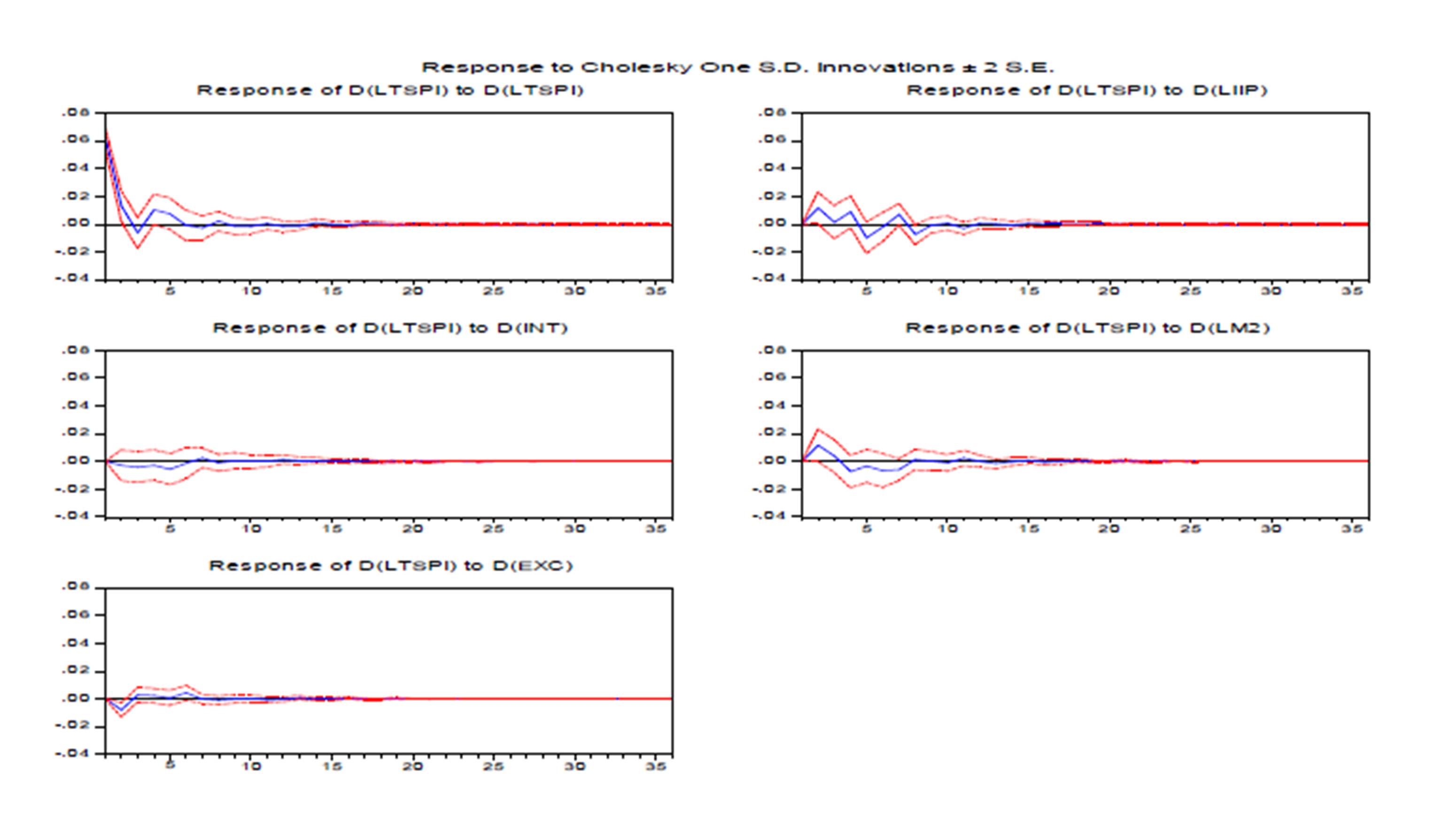
Figure1: Impulse response to non-factorized one S.D. innovation ∓ 2 S.E; 1) response of D(LTSPI) to D(LTSPI); 2) response of D(LTSPI) to D(LIIP); 3) response of D(LTSPI) to (LINT); 4) response of D(LTSPI) to D(M2); 5) response of D(LTSPI) to D(EXC)
Figure 1 reported the results of LTSPI impulse responses to a set of macroeconomic variables. Results indicate that LTSPI response to its own shock is significant and negative in the 2nd period. But, the response of LTSPI to shock from LIIP is significant and positive in the 8th period then will die out maximum within the 20th period. While, LTSPI response to shock from LM2is significant and negative in the 2nd period. Finally, the response of LTSPI to a shock from EXC has a significant and negative effect in the 2nd period then dies out maximum within the 20th period.
Conclusion
The aim of this study is to provide empirical evidence and to elucidate the dynamic relationship between the whole Turkish stock price index and macroeconomic variables, for a wiser time span from January 2002 to December 2013 (restructuring period).
The findings reveal that the long-run relationship between the whole Turkish stock price index and macroeconomic variables namely: (Short-term interest rate (SINT), money supply (M2), exchange rate (EXC), and index of industrial production (IIP) as a proxy of economic activity) is maintained. Dummy variables were added to the model to overcome the effect of monetary policy changes and world crisis.
Moreover, the existence of long-run equilibrium relationship between whole share price index and a set of macroeconomic variables was a result of the negative sign of the residual in the estimated ECT. Hence, the coefficient for ECT indicates that the Turkish stock market corrects its previous disequilibrium due to positive or negative shocks in one period at an adjustment speed of 4.449 percent monthly. Also, the result indicates a robust response of Turkish stock price to a shock of exchange rate over time period. Furthermore, the impulse response finding indicates that shocks on the Turkish stock market will die out maximum within the 20th period. Therefore, policymakers should take into account the use of the exchange rate as a tool in monetary policy because of its robust influence on the whole Turkish stock market. As long as the Central Bank intervention into the foreign exchange market in order to increase exchange reserves with respect to capital inflow.
Note:
Deterministic trend: Perron, 1989).
The expected negative sign: For instance, if Yt−1 and Xt−1 their long-run values are estimated by long-run system with a positive disequilibrium error. Consistency, this period Yt−1 and Xt−1 falls in order to move back to their long-run equilibrium values (ΔXt and ΔYt will be negative).
(adsbygoogle = window.adsbygoogle || []).push({});
References
1.Adrangi, B &Chatrath, A. (2007)‘Inflation, Output, and Stock Prices: Evidence from Brazil’, the Journal of Applied Business Research. Vol. 18, No,1.
2.Ahmet, B &Abdioglu, H. (2010)‘The Causal Relationship between Stock Prices and Macroeconomic Variables A Case Study for Turkey’,International Journal of Economic Perspectives,Vol 4, Issue 4, 601-610.
Google scholar
3. Buyuksalvarci, A. (2010) ‘The effects of macroeconomics variables on stock returns: Evidence from Turkey’,European Journal of Social Sciences, 14(3), 70-83.
4. Cağli, Ç. Halaş, U.Taşkin, D. (2010) ‘Testing Long-Run Relationship between Stock Market and Macroeconomic Variables in the Presence of Structural Breaks: The Turkish Case’,International Journal of Finance and Economic, ISSN 1450-2887, Issue, 48.
5.Chen, S, J, Roll, F, Ross, S, A (1986) ‘Economic Forces and the Stock Market’,Journal of Business, Vol 59, 3, PP 505-523.
6.Choi, J, Elyasiani, E. Kopecky, K. (1992) ‘The Sensitivity of Bank stock Return to Market, Interest and Exchange Rate Risks’,Journal of Banking and Finance, 16, PP 983-1004.
7.Civcir, I. (2009)‘Inflation Targeting and the Exchange Rate; Does it matter in Turkey? Journal of Policy Modeling.JPO-5833; of page 16.
8.Deb, G. Mukherjee, J.(2008) ‘Does stock market development cause economic growth? A time series analysis for Indian economy’,International Research Journal ofFinance and Economics. ISSN 1450-2887 issue 73.
9.Enders, W. (2004) Applied Econometric Time Series, second edition. John Wiley & Sons Inc, New York.
10.Erdem, C, Arslan, C. K, &Erdem, M, S. (2005) ‘Effects of Macroeconomic Variables on Istanbul stock exchange indexes’, Applied Financial Economics, 15, 987-994.
Publisher – Google Scholar
11.Ewing, B. (2002) ‘Macroeconomic News and the Returns of Financial Companies’,Managerial and Decisions Economics, Vol 23, 8, PP 439-446.
Google Scholar
12. Groenewold, N. Fraser, P. (1997) ‘Share Prices and Macroeconomic Factors’,Journal of Business Finance and Accounting, Vol 24, 9&10, PP 1367-1383.
Google Scholar
13. Humpe, A. Macmillan, P. (2009) ‘Can Macroeconomic Variables Explain Long-run Stock Market Movements?A Comparison of the U.S. and Japan’,Applied Financial Economics, 19 (2), 111-119.
Publisher – Google Scholar
14.Ibrahim, M. Aziz, H. (2003) ‘Macroeconomic variables and the Malaysian equity market’,Journal of Economic Studies. 30, 1: 6-27.
Publisher – Google Scholar
15.Issahaku, H, Ustarz, Y &Domanban, P. (2013). Macroeconomic Variables and Stock Market Returns in Ghana: any causal link? Asian Economic and Finance Reviewer, 3(8): 1044-1062.
16.Johansen, S. (1988) ‘Statistical analysis of Cointegrationvectors’,Journal of Economic Dynamics and Control.12, 231-254.
Publisher – Google Scholar
17.Joseph, F. Jakkaphong, J. (2014) ‘Selected macroeconomic variables and stock market movements empirical evidence from Thailand’, Contemporary economics, Vol.8(2), pp.157-174.
Google Scholar
18.Kasman, S. (2003) ‘The Relationship between Exchange Rates and Stock prices: a causality analysis: Evidence from Turkey’,DokuzEylülüniversitesiSosyalBilimlelEnstitüsüDergisiCilt 5 sayi, 2.
Google Scholar
19. Kose, M. A., Parasad, E. S., ROGOFF, K. WEI, S. (2006) ‘Financial globalization. Are appraisal’,NBER Working Paper No.12484. Cambridge, MA: NBER.
20. Lajeri, F. Dermine, J. (1999) ‘Unexpected Inflation and Bank Stock Returns: The Case of France’,Journal of Banking and Finance, 23, PP 939-953.
Google Scholar
21.Lekobane, S. Khaufelo, K. (2014), ‘Do Macroeconomic Variables Influence Domestic Stock Market Price Behaviour in Emerging Markets? A Johansen Cointegration Approach to the Botswana Stock Market’, Journal of Economics and Behavioral Studies Vol.6 (5), pp.363-372.
Google Scholar
22.Lütkepohl, H. (2005) New Introduction to Multiple Time Series Analysis. Second editions, Springer, Berlin.
Publisher – Google Scholar
23.Maysami, C., Howe, L.Hamzah, M. (2004) ‘Relationship between macroeconomic variables and stock market indices: Cointegration evidence from stock exchange of Singapore’s all-S sector indices’,JurnalPengurusan, 24, 47-77
Google Scholar
24.Merikas, A. Merika, A. (2006) ‘Stock Responses to Real Economic Variables: The Case of Germany’,Managerial finance, Vol 32, 5, PP 446-450.
Google Scholar
25.Muradoglu, G. Metin, K.Argae, R. (2001)‘Is there a long-run relationship between stock returns and monetary variables: Evidence from an emerging market’,Applied Financial Economics,7(6), 641-649.
Google Scholar
26.Nelson, C. Plosser, C. (1982) ‘Trend and Random Walks in Macroeconomics Time Series’,Journal of Monetary Economics, 10 (2), 139-162.
27.Perron, P. (1989) ‘The great crash, the oil price shock, and the unit root hypothesis’,Econometrica, 57, pp.1361-1401.
Publisher – Google Scholar
28. Pilinkus, D. (2009)‘ Stock Market and Macroeconomic variables: Evidences from Lithuania’,Economic and Management ISSN 1822-6515.
29.Rahman, L. Uddin, J. (2009)‘ Dynamic Relationship between Stock Prices and Exchange Rates: Evidence from Three South Asian Countries’,International Business Research.Vol.2, N2.
Google Scholar
30. Raymond, K. (2009) ‘Is There a Long Run Relationship Between Stock Prices and Monetary Variables? Evidence from Jamaica’, Financial Stability Department Bank of Jamaica.
Google Scholar
31.Rjoub, H. (2012) ‘Stock prices and exchange rate dynamics: Evidence from emerging markets’,African Journal of Business and Management, 6 (13).
Google Scholar
32.Yartey, C.(2008)‘The determinants of stock market development in emerging economies: is South Africa different? IMF Working Paper No.WP/08/32.
Google Scholar
33. Zivot, E. Andrews, K. (1992) ‘Further Evidence on the Great Crash, the OilPrice Shock, and the Unit Root Hypothesis’,Journal of Business and Economic Statistics, 10 (10), pp. 251—70.
Publisher – Google Scholar
34.Zugul, M.Sahin, C. (2009)‘ISE 100 Index and the Relationship Between Some Macroeconomic Variables’, An Application Oriented Review, Academic Overview of e-journals, 16.