Introduction
Since the path-breaking work of Akerlof (1970), Spence (1973), Nelson (1970; 1974) and Stiglitz (1975), hundreds of theoretical articles have explored the economics of information in general and signaling in particular. A detailed review of this literature is well beyond the scope of this research, and others have provided excellent review articles (Riley, 2001; Spence, 2002; Stiglitz, 2000; 2002).
We address just one aspect of this issue here, the necessity of sellers, in the face of asymmetric information, to signal the level of quality of their product to buyers. This is the now familiar “lemons” problem, where failure to signal quality and to charge more for it would drive higher quality sellers from the market, leaving only low quality “lemons” and, in extreme circumstances, cause a market not to exist.
Empirical work testing for the existence of signaling in markets is much scarcer than its theoretical counterparts. We will review some of this literature in the next section, but by way of introduction, we would simply note that even the empirical signaling literature is virtually silent on the dynamics of convergence to a Spence signaling equilibrium, the adjustments over time by sellers and buyers through quality signals and purchasing behavior.
As we will see in the next section, a growing body of empirical work has demonstrated that many products in the face of asymmetric information about quality are not “lemons.” These studies, using regression analysis for the most part, show that a statistical relationship exists between product price and quality attributes of the product, suggesting successful signaling on the part of sellers. In most of these studies, however, signaling is incomplete, as much of the variance in a product’s price remains unexplained, even after taking quality signals into account. Furthermore, few empirical studies demonstrate that the degree of successful product signaling increases over time, through learning that leads to a convergence to a signaling equilibrium.
This is the contribution of this paper. Using data on a particular market characterized by asymmetric information, a wine market, we show that over time, for the same set of wines, the statistical fit of regressions of price on quality improves. Moreover, there exists a statistically significant time trend of the goodness of fit of annual signaling regressions. To our knowledge, this is the first statistical evidence of convergence toward a signaling equilibrium.
Literature Review
We limit our more detailed review of empirical literature to the work on signaling in product markets only, not services. For example, much empirical work exists on signaling in markets for financial and labor market services, including educational screening. For an introduction to much of this related literature, see Riley, 2001; Spence, 2002; and Stiglitz, 2000; 2002.
Bond (1982) provided the first direct test of Akerlof’s “lemons” model, when he examined the market for used pickup trucks with data from the 1977 Truck Inventory and Use Survey. After controlling for mileage and model year, Bond tested for the statistical equality of mean engine maintenance across the two groups, original-owner and purchased-used groups. He found no evidence that used pickups required more maintenance than pickups purchased new, i.e., signaling had ensured that used pickup trucks were not “lemons.”
Other researchers have tried to link quality to particular signals. Pricing and advertising have received much attention in the theoretical literature (e.g., Friedman, 1967; Nelson, 1970; 1974; Monroe, 1973; Kihlstrom and Riordan, 1984; Milgrom and Roberts, 1986; Bagwell and Riordan, 1991; Bagwell, 1992; Caves and Greene, 1996; Jones and Hudson, 1996). Early survey research suggested that consumers believe that quality and price have positive correlation (Leavitt, 1954; Tull et al., 1964; Gabor and Granger, 1966; McConnell, 1968) Statistical analysis, however, often concluded that the relationship is weak, at best (Morris and Bronson, 1969; Sproles, 1977; Riesz, 1978; 1979; Geistfeld, 1982; Gerstner, 1985; Hjorth-Andersen, 1991).
Some of the more recent studies are instructive. For example, Gerstner (1985) used data on prices and ordinal quality rankings to estimate rank correlation coefficients of price and quality for 145 products. For only 28% of the products could he reject the null hypothesis of no correlation at the 5% level of significance. Similarly, Hjorth-Andersen (1991) used Consumer Reports data and rank correlation methods and found stronger price-quality relationships, with positive correlations dominating negative ones 2-1, although a finding of 1/3 negative correlations was still a little disturbing.
Warranties from sellers can signal quality to buyers. Wiener (1985) used Consumer Reports data on consumer durables and motor vehicles to test the relationship between better warranties and higher quality, measured as product reliability. With three reliability categories and two warranty categories, Wiener concluded that, indeed, a product’s warranty is an accurate signal of its reliability.
Rosenman and Wilson (1991), in an analysis of the Washington cherry market, moved the signaling literature in the direction of our work. Quality differentials for cherries are related mainly to size. Many sellers sort cherries into size categories and receive a higher price for boxes of larger cherries. One heterogeneous size category exists, however. Rosenman and Wilson hypothesized that a signaling equilibrium exists if sellers who don’t sort their cherries receive a higher price in the heterogeneous category than sellers who do sort, i.e., non-sorting sellers signal higher quality (larger average size) by not sorting. By regressing price on seller characteristics and a sorting dummy variable, they found a negative and statistically significant coefficient on the sorting dummy. With R-square statistics ranging from 0.12 – 0.19, they concluded that a signaling equilibrium existed in cherries, i.e., cherries are not “lemons.”
More recently, empirical researchers have addressed signaling in wine markets. Most of this research examined markets for Bordeaux wine. Dubois and Nauges (2009) used chateaux panel data to examine the effect of expert opinion and unobserved quality on the en primeur price of Bordeaux wine, the price established by an informal market when the wine is still in the barrels, a potential signal of the wine’s quality. They argued that unobserved true quality, more likely known by producers, and likely correlated with expert quality rating, might cause omitted variable bias. The authors concluded that failure to control for this omitted variable bias can lead to an overstatement of the effect of expert opinion on en primeur price.
Hadj and Nauges (2007) also examined Bordeaux en primeur wines. They found a statistically significant and quantitatively important rank-reputation premium attached to different Bordeaux wines. By contrast, current and lagged expert quality rating, and the Wine Spectator vintage rating, while statistically significant, had small quantitative impacts on en primeur prices. They also found that en primeur prices and current quality rating and reputation variables explained 86% of the variance in market price, and concluded that the en primeur price was an effective signal of the market price.
Continuing the analysis of French wine markets, Hadj et al. (2008) also examined the impact of expert opinion on en primeur prices of Bordeaux wines. Instead of focusing on the effect of different magnitudes of the expert rating across a large panel data set, as in other studies, they looked at the “treatment effect” of the rating itself. Using the fact that wine expert Robert Parker did not review Bordeaux wines before en primeur prices were established for the 2002 vintage, as he had in other years, the authors were able to conclude that the “Parker effect” averaged 2.8 euros per bottle. Mahenc (2004) and Mahenc and Meunier (2006) have also explored signaling in these markets.
Signaling in U.S. wine markets was examined by Miller et al. (2007) and Miller et al. (2011). Miller et al. (2007) used a limited sample of 2001 California cabernet sauvignon wines reviewed and rated in a print issue of the Wine Spectator. They regressed a measure of a wine’s price on a quality rating, number of cases produced and a measure of the storage ability (i.e., cellar life) of the wine. Overall, the regression explained about 45% of the variance in price, so they concluded that signaling through quality rating and production quantity was occurring successfully in the market for 2001 California cabernet sauvignon. In an Akerlof sense, these wines are not lemons, but the authors stopped short of drawing the conclusion made by Rosenman and Wilson (1991) that this constituted evidence of a signaling equilibrium. They concluded that because much of the sample’s variance in wine price remained unexplained by quality signals, the possibility of further seller and buyer adjustments toward a signaling equilibrium might be expected to occur over time. Using similar data, Miller et al. (2011) showed that the R-square statistic increased in three pairs of years in the early 2000s in regressions of the price of a wine on its quality signals, but they provided no statistical evidence of a convergence to a signaling equilibrium.
Data and Methods
Our data consist of observations on cabernet sauvignon wines produced in California over the years 2001 through 2005 and reviewed in Wine Spectator, accessed online. The variables collected are price, measured as the release price, the number of wine cases produced for the year, whether the wine is labeled as “reserve,” and whether or not the wine is produced using grapes from the Napa Valley of California.
Because we focus on signaling and purchasing adjustments over time, we need a common set of wines. This presents a major challenge for this kind of research, as a large amount of attrition in the specific wines offered for sale occurs from one year to the next. In fact, a specific wine might appear in the data set one year, but not for the next year or two, only to reappear in later years. Reasons for such attrition are varied, but include not offering the wine for sale in a given year due to production or quality issues, relabeling or rebranding of the wine, or wines not reviewed by Wine Spectator in a particular year.
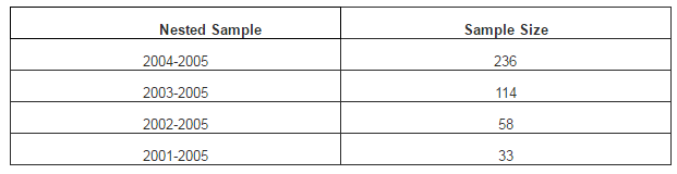
In order to develop common sets of wines in the data set, given the year-to-year attrition, we use a nested sample approach. We began with the years 2004 and 2005 and identified 236 wines in common across those two years. The next nested sample is for the years 2003, 2004, and 2005. The wines in 2003 are compared to the common wines identified for the years 2004 and 2005 to again develop a common set of wines for those years, resulting in 114 wines in this sample. We repeated the process, adding one year at a time, until all years appear in the nested sample. The resulting samples decline in size as each additional year is added. The other sample sizes are 58 wines for 2002 through 2005 and 33 wines for years 2001 through 2005. These sample sizes are displayed in Table 1.
Table 1: Nested Sample Sizes
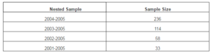
As seen above, adding additional years to a nest further increases the attrition. In other exploratory work, we added years 2000, 1999 and 1998, and the resulting sample sizes shrunk to 21, 17 and 13 respectively. We limited our smallest sample to n=33, for years 2001 to 2005. We show descriptive statistics for the variables in the various nested samples in Table 2.
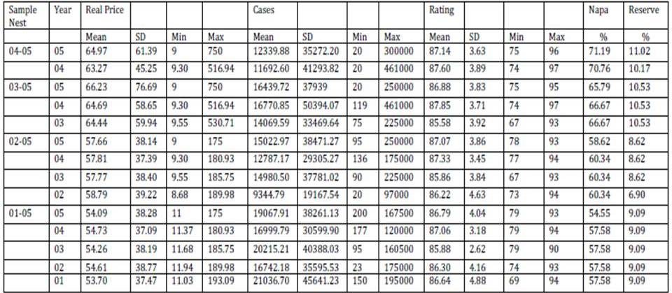
Table 2: Descriptive Statistics for the Nested Samples
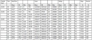
SD denotes standard deviation.
Nothing dramatic appears in these statistics, but some characteristics warrant a brief discussion. As seen in the Real Price Mean column, these are not inexpensive wines, with mean prices over $50 in all years. As we move down the table, from larger to smaller samples (04-05 to 01-05), mean prices decline. This is likely from high-price wines leaving the sample. For example, the maximum price in the 04-05 and 03-05 samples, the largest samples, is $750, while the maximum price in the 01-05 and 02-05 samples, the smaller samples, is about $190. Much less change occurs in minimum prices, which are always in the $9-$12 range. The lower maximum prices in the smaller samples are associated with lower variation in the price variable. For example, the standard deviation divided by the mean for 2005 in the 04-05 samples is 0.94 and 1.16 in the 03-05 samples. For the same year in the 01-05 samples, it falls to 0.71. For the 02-05 samples, it is 0.66.
The wines in our samples, on average, are produced in reasonably large volumes. Mean number of cases produced ranges from about 9,000 to 21,000 cases. Small production wineries exist in all years and in all samples, with minimum cases ranging from 20 to 200 cases, depending on the year. On the other hand, large production wineries are present in the samples, as well, with maximum cases produced ranging from 97,000 to 461,000 cases. Comparing standard deviations to means in the cases variable indicates much larger variation than that in wine prices, with coefficients of variation commonly in the neighborhood of 2 — 3.5. Also mean cases produced generally rises as the sample size gets smaller. For example, annual mean production ranges from 16,742 to 21,037 cases in the 01-05 sample, and 11,693 to 12,340 in the 04-05 samples.
Quality ratings in our samples, on average, are about 85-88, a Wine Spectator rating indicating “very good wines with special qualities.” While the quality rating ranges from a low of 67 to a high of 97, depending on the sample and year, in general the overall variation in quality rating is low, with coefficients of variation around 3-5%.
The final two columns of Table 2 show the percent of the wines from the Napa region and the percent with a “reserve” designation. It appears that the smaller samples contain a smaller proportion of wines from the Napa region and a slightly smaller proportion with reserve designation.
For the purposes of interpretation of results presented below, we can summarize these descriptive statistics as indicating the following. As the nested sample increases in length, sample size decreases. As the sample gets smaller, “outliers” disappear. For example, the maximum price falls from $750 to $190. The minimum price rises from $9 to $11-$12. The maximum number of cases declines from 461 thousand to 195 thousand. The maximum rating falls from the high 90s to the low 90s. This is associated with a reduction in the mean quality rating, although the reduction is not large. The mean number of cases rises. The proportion of wines not from Napa rises and the proportion with reserve designation falls. These developments are not inconsistent with convergence to a signaling equilibrium, where the convergence involves attrition of all but the more familiar wines over time. These results, however, are for the sample aggregates. In the following, we use regression analysis in an attempt to find an improvement in the relationship of individual wine prices to the wine’s quality attributes over time.
Our analysis uses a two-step process. In the first step we estimate, for each year in each nested sample, a regression equation relating the price variable to its signaled quality attributes. In the second step, we use goodness of fit statistics such as the R-square or mean square error from each regression estimated in the first step as the dependent variables in another regression. The explanatory variables in this regression are dummy variables for each year, or alternatively each nest, and a trend variable indicating the position of the particular year in a nested sample. If signaling occurs, this trend variable should be positive and statistically significant, as a greater explained variation in wine prices is captured by an improved goodness of fit statistic. The details of both steps in the analysis and the regression results are described in more details below.
Research Results
The First Step: The Individual Year Regressions
First, we estimate the regression equation for each year in each nested sample. These estimations are performed using the regression procedure and ordinary least squares in PC SAS version 9.2. The regression equation is a natural logarithm transformation. The dependent variable is the logarithm of the wine’s release price in real terms. The explanatory variables include natural logarithms of the number of cases produced and the wine’s quality rating from Wine Spectator. The number of cases captures production factors for the wine, and perhaps desirable demand characteristics related to limited supply. Quality rating provides an independent evaluation of the wine’s quality. In addition, two dummy variables are included to capture other dimensions of the wine’s quality. These variables, reserve and Napa, have the value of one if the wine is designated as a reserve wine and if the grapes used in the wine are grown in the Napa Valley of California, respectively. The specific form of the regression equation is shown in equation 1.
(1) ln (price) = constant + 1ln(number of cases) + 2ln(quality rating) + 3(Napa)+ 4(reserve) +
We have a priori expectations for the signs of the coefficients in the regression equation shown above. The number of wine cases is expected to be inversely related to the price of the wine, because the greater the quantity available on the market, the greater its depressing impact on price. In addition, some wine buyers prefer exclusive wines limited in quantity, so small production could positively influence willingness to pay.
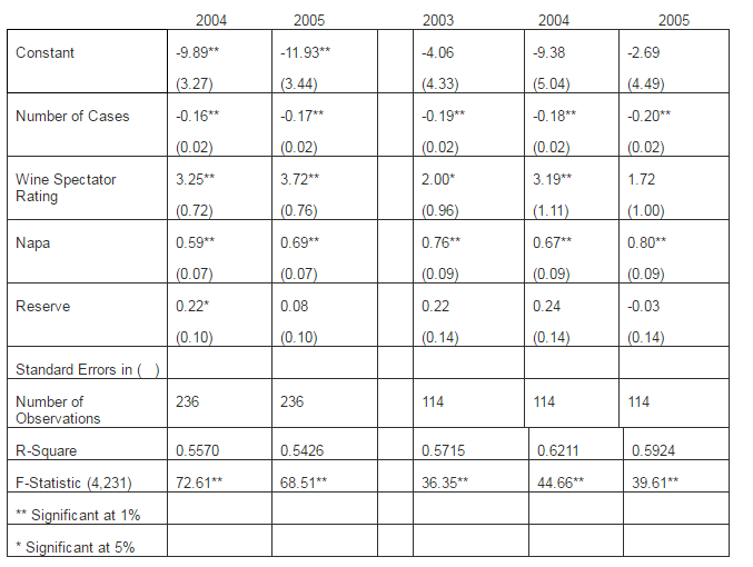
We expect wine quality rating is directly related to the wine’s price. Both dummy variables also reflect dimensions of the wine’s quality, and as such are expected to directly impact the wine’s price. The results from these regressions are displayed in Table 3.
Table 3: Individual Year Regression Results
2004-2005 Sample 2003-2005 Sample
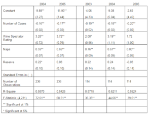
Table 3: (Continued)
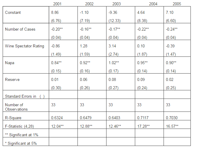
2002-2005 Sample
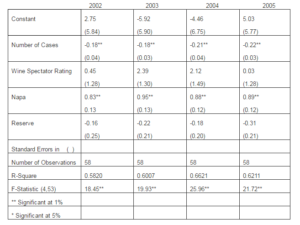
2001-2005 Sample

Interpretation of the regression results in Table 3 is reasonably straightforward. Each regression has a statistically significant R-square statistic, ranging from a low of 0.54 for 2005, in the 2004-2005 nested samples, to a high of 0.71 for year 2004, in the 2001-2005 nested samples. The Number of Cases variable and the Napa dummy are of the right sign and statistically significant at the 1% level throughout. The reserve dummy is rarely significant, and the Wine Spectator Rating is significant only in samples with reasonably large numbers of observations, nested samples 2004-2005 and 2003-2005. At smaller sample sizes, we expect that lack of variation in price and rating might be the cause of this absence of statistical significance.
The Second Step: The Regression of the Goodness of Fit Statistics
In the first part of our second step, we examine the relationship between an individual year’s estimated R-square within a nested sample to that year’s position in the nested sample. If signaling of the wine’s quality occurs, the position of that year within the nested sample should have a significant impact on that year’s R-square. Ours is a second-best approach, however, necessitated by the attrition of wines from a common sample as years advance. In a world of perfect data, we would have, say, 20 years of data on a large number of the same wines. In reality, the common set of wines diminishes in number much more rapidly.
More formally, the regression at this step in the analysis uses the R-squares from the regressions estimated in the first step of the analysis as the dependent variable observations. One of the explanatory variables is a trend variable capturing a particular year’s position in its nested sample. This variable is labeled “year in sample.” For example, if the particular year is the first in the nested sample, the year in sample variable has the value of one. If the year is the second in the nested sample, this variable takes on the value of two, and so on. The other explanatory variables are dummy variables for each year 2001 through 2004 with 2005 the omitted year.
(2) R-square = constant + 1(year in sample) + 2D2001 + 3D2002 + 4D2003 + 5D2004 + 6D2005 +
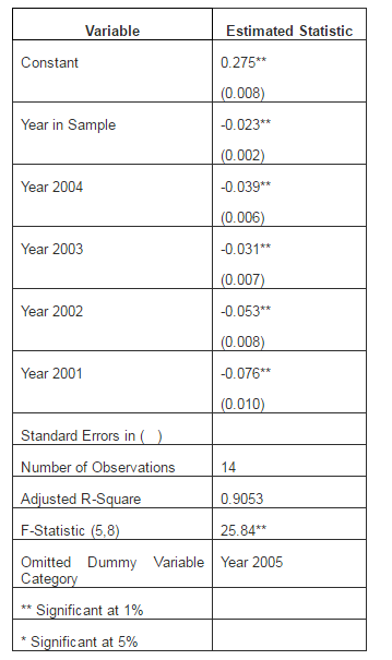
There are a total of 14 observations, driven by the 14 R-square values estimated in the first step of the analysis. The regression results are shown in the leftmost portion of Table 4. The R-square for the regression is 0.94. The coefficient on the year in sample variable is statistically significant at a 1% level and has the expected positive sign. The result indicates that as the year progresses through the nested sample, it has a positive impact on the R-square. Indirectly, since the R-squares are from regressions using the wine release price as the dependent variable, this result implies that, as the year progresses through the nested sample, we explain a greater proportion of the variations in the wine’s price by its quality signals. Such is the result over time of adjustments in signaling and purchasing behavior. Additionally, each of the four dummy variables for the individual years and the constant of the regression are statistically significant at a 1% level.
Table 4: R-Square Regressions Results
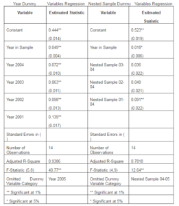
In the rightmost portion of Table 4, we present results with a different set of dummy variables. As can be seen in Table 3, the R-squares of the individual regressions increase in general as the length of the nested sample increases and the number of observations decreases. In this regression, we include dummies to account for nest effects on the particular regression’s R-square. The R-squares in the sample 2001-2005 are higher than the others by a statistically significant amount. While the coefficient on the trend variable falls in magnitude in this regression compared to the regression with year dummies, the coefficient remains statistically significant at the 5% level.
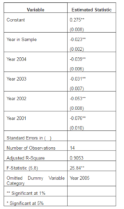
As mentioned above, an upward drift in the R-squared statistic exists in our nested samples as the sample size decreases. We attempt to control for this somewhat with the nest dummy variables in the regression shown in the right portion of Table 4. Alternatively, we can use a different goodness of fit measure, mean squared error, to address the difference in sample size. Defined as the sum of the squared errors (residuals) divided by the sample size, this statistic controls for sample size in its very definition. Table 5 shows the results from regression of mean squared error on the year in sample trend variable and year dummies. This regression is analogous to the regression in the left part of Table 4, but with a different goodness of fit dependent variable. Again, as with the R-square regression, the coefficient of the year in sample trend variable (now negative in sign) is statistically significant at the 1%, indicating a reduction in the mean squared error as year in sample increases.
Table 5: Mean Square Error Regression Results
Conclusions
While some empirical work tests for the existence of Akerlof’s “lemons” problem, there has been very little in the economics of information literature on the dynamic issue of convergence to a Spence signaling equilibrium. We have attempted to provide some statistical evidence here. In the process, we have discovered the main challenge in this type of work, at least in the way we have approached it. This is the problem of attrition in finding a common set of products as the number of years in a sample increases.
We have attempted to address this problem with our nested sample procedure and time trend analysis on goodness of fit statistics, but in the end, there are problems with this approach as well. We noticed, for example, a general upward drift in the average R-square statistics as the nested sample increases in length and, in turn, the number of observations in it falls. This change in R-square appears to be greater across the nested samples than within the samples. We controlled for this with “nest” dummies and with use of the mean square error measure that takes account of sample size.
Yet nagging questions remain. While descriptive statistics for our samples tell a story not inconsistent with convergence to a signaling equilibrium, and our statistical tests for improvement in ability to relate price to quality attributes suggest convergence, as well, the problem of untangling attrition of wines from the sample from improvement in consumer and produces assessment of them remains. In the future, we hope to examine the nature of this attrition of wines in wine markets, which itself is a form of signaling behavior.
References
Akerlof, G. (1970). “The Market For ‘Lemons:’ Quality Uncertainty and the Market Mechanism,” Quarterly Journal of Economics, 84, 488-500.
Publisher – Google Scholar
Ali, H. H. & Nauges, C. (2007). “The Pricing of Experience Goods: The Example of en Primeur Wine,” American Journal of Agricultural Economics, 89, 91-103.
Publisher – Google Scholar
Ali, H. H., Lecocq, S. & Visser, M. (2008). “The Impact of Gurus: Parker Grades and En primeur Wine Prices,” The Economic Journal, 118, 158-173.
Publisher – Google Scholar
Bagwell, K. (1992). “Pricing to Signal Product Line Quality,” Journal of Economics & Management Strategy, 1, 151-74.
Publisher – Google Scholar
Bagwell, K. & Riordan, M. H. (1991). “High and Declining Prices Signal Product Quality,” American Economic Review,81, 224-239.
Publisher – Google Scholar
Bond, E. W. (1982). “A Direct Test of the ‘Lemons’ Model: The Market for Used Pickup Trucks,” American Economic Review, 72, 836-840.
Publisher – Google Scholar
Caves, R. E. & Greene, D. P. (1996). “Brands’ Quality Levels, Prices, and Advertising Outlays: Empirical Evidence on Signals and Information Costs,” International Journal of Industrial Organization, 102, 179-221.
Publisher – Google Scholar
Dubois, P. & Nauges, C. (2009). “Identifying the Effect of Unobserved Quality and Expert Reviews in the Pricing of Experience Goods: Empirical Application on Bordeaux Wine,” International Journal of Industrial Organization, AAWE Working Paper No. 10.
Publisher – Google Scholar
Friedman, L. (1967). ‘Psychological pricing in the food industry, Prices: Issues in Theory, Practice, and Public Policy,’ Phillips, A. and Williamson, O. I. (eds), University of Pennsylvania Press, Philadelphia, PA.
Gabor, A. & Granger, C. W. J. (1966). “Price as an Indicator of Quality: A Report on an Inquiry,” Economica, 33, 43-70.
Publisher – Google Scholar
Geistfeld, L. V. (1982). “The Price-Quality Relationship — Revisited,” Journal of Consumer Affairs, 16, 334-335.
Publisher – Google Scholar
Gerstner, E. (1985). “Do Higher Prices Signal Higher Quality?,” Journal of Marketing Research, 22, 209-215.
Publisher – Google Scholar
Hjorth-Andersen, C. (1991). “Quality Indicators in Theory and Fact,” European Economic Review, 35, 1491-1505.
Publisher – Google Scholar
Jones, P. & Hudson, J. (1996). “Signaling Product Quality: When is Price Relevant?,” Journal of Economic Behavior and Organization, 30, 257-266.
Publisher – Google Scholar
Kihlstrom, R. E. & Riordan, M. H. (1984). “Advertising as a Signal,” Journal of Political Economy, 92, 427-50.
Publisher – Google Scholar
Leavitt, H. J. (1954). “A Note on Some Experimental Findings about the Meaning of Price,” Journal of Business, 41, 439-444.
Publisher
Mahenc, P. (2004). “Influence of Informed Buyers in Markets Susceptible to the Lemons Problem,” American Journal of Agricultural Economics, 86, 649-659.
Publisher – Google Scholar
Mahenc, P. & Meunier, V. (2006). “Early Sales of Bordeaux Grands Crus,” Journal of Wine Economics, 1, 57-74.
Publisher – Google Scholar
McConnell, D. J. (1968). “An Experimental Examination of the Price-Quality Relationship,” Journal of Business, 41, 439-444.
Publisher – Google Scholar
Milgrom, P. & Roberts, J. (1986). “Price and Advertising Signals of Product Quality,” Journal of Political Economy, 94, 796-821.
Publisher – Google Scholar
Miller, J. R., Genc, I. & Driscoll, A. (2007). “Wine Price and Quality: In Search of a Signaling Equilibrium in 2001 California Cabernet Sauvignon,” Journal of Wine Research, 18, 35-46.
Publisher – Google Scholar
Miller, J. R., Stone, R. W., Stuen, E. T. & Barker, M. (2011). ‘Tests for Convergence Toward a Signaling Equilibrium: The Case of California Cabernet Sauvignon,’ Journal of Business and Economic Studies, 17, 65-79.
Google Scholar
Monroe, K. B. (1973). ‘Buyers’ Subjective Perception of Price, Perspectives in Consumer Behavior,’ Kassarijian, H. H. and Robertson, T. S. (eds), Scott, Foresman, Glenview.
Morris, R. T. & Bronson, C. S. (1969). “The Chaos in Competition Indicated by Consumer Reports,” Journal of Marketing, 33, 26-43.
Publisher – Google Scholar
Nelson. P. (1970). “Information and Consumer Behavior,” Journal of Political Economy, 78, 311-29.
Publisher – Google Scholar
Nelson, P. (1974). “Advertising as Information,” Journal of Political Economy, 81, 729-54.
Publisher – Google Scholar
Riesz, P. C. (1978). ‘Price Versus Quality in the Marketplace, 1961-1975,’ Journal of Retailing, 54, 15-28.
Google Scholar
Riesz, P. C. (1979). “Price-Quality Correlations for Packaged Food Products,” Journal of Consumer Affairs, 13, 236-47.
Publisher – Google Scholar
Riley, J. G. (2001). “Silver Signals: Twenty-Five Years of Screening and Signaling,” Journal of Economic Literature, 39, 432-478.
Publisher – Google Scholar
Rosenman, R. E. & Wilson, W. W. (1991). “Quality Differentials and Prices: Are Cherries Lemons?,” The Journal of Industrial Economics, 39, 649-668.
Publisher – Google Scholar
Spence, M. (1973). “Job Market Signaling,” Quarterly Journal of Economics, 87, 355-374.
Publisher – Google Scholar
Spence, M. (2002). “Signaling in Retrospect and the Informational Structure of Markets,” American Economic Review,92, 434-459.
Publisher – Google Scholar
Sproles, G. B. (1977). “New Evidence on Price and Product Quality,” Journal of Consumer Affair, 11, 63-77.
Publisher – Google Scholar
Stiglitz, J. E. (1975). “The Theory of Screening, Education and the Distribution of Income,” American Economic Review,65, 283-300.
Publisher – Google Scholar
Stiglitz, J. E. (2000). “The Contributions of the Economics of Information to Twentieth Century Economics,” The Quarterly Journal of Economics, 115, 1441-1478.
Publisher – Google Scholar
Stiglitz, J. E. (2002). “Information and the Change in the Paradigm in Economics,” American Economic Review, 92, 460-501.
Publisher – Google Scholar
Tull, D. R., Boring, R. A. & Gonsior, M. H. (1964). “A Note on the Relationship of Price and Imputed Quality,” Journal of Business, 37, 186-191.
Publisher – Google Scholar
Wiener, J. L. (1985). “Are Warranties Accurate Signals of Product Reliability?,” Journal of Consumer Research, 12, 245-250.
Publisher – Google Scholar