Introduction

Solution architectures are essential for companies to enable value generation and increase the efficiency of processes related to design and implementation of technology solutions (Arango Serna et al., 2015). As Fig. 1  shows, a technology solution’s design considers solution architectures from which are derived one or more alternatives that represent different options for the technology solution (Pena et al., 2017a). An alternative has a set of solution components that represent technology functionalities such as information systems (Arango Serna et al., 2015; Pena et al., 2017b), which in turn can have particular variables such as benefits and costs associated with them and that must be considered to calculate the alternative’s financial indicators using cost-benefit models (Brealey et al., 2011; Irani et al., 2006; Pena et al., 2017a). Financial indicators are indispensable for determining the feasibility of the technology solution, analyzing its possible risks, and for justifying any investment (Irani et al., 2006; Neufville and Scholtes, 2011). These financial indicators must consider uncertainties derived from unpredictable events such as changes in requirements to identify positive or adverse consequences of IT investments (Neufville and Scholtes, 2011; Pena et al., 2017a).

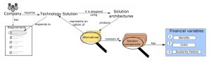
Fig. 1: Solution architecture approach

Once alternatives are defined, a company has the crucial task of selecting the one that is most convenient for implementing the technology solution (Pena et al., 2017a). To choose an alternative, companies commonly compare the alternatives’ financial indicators (Brealey et al., 2011; Pena et al., 2017a). Although comparison of alternatives is valuable, it is important to consider the financial indicators at the component level because they include particular financial variables, economic factors, and unpredictable events (Pena et al., 2017a) that support analyses such as comparison of the profitability between components of various alternative solutions (Pena et al., 2017a).

Although there is an extensive literature about cost-benefit models addressed to technology solutions (Apfel and Smith, 2003; Cormier, 2010; Kazman et al., 2002), most of these models are directed at overall IT investments and have a high level of granularity[i]  (Mead et al., 2009; Pena et al., 2017b) that limits the detailed cost-benefit analysis required for solution architectures.  Consequently, financial indicators may not accurately indicate valuation due to the omission of specific variables (Mead et al., 2009; Pena et al., 2017b),  it may be difficult to identify financial indicators at the component level which could limit comparisons of components (Pena et al., 2017a), and uncertainty at the component level could impact financial indicators. This study defines FINFLEX-CBMC, an innovative cost-benefit model that supports financial analysis of alternatives and solution components in solution architectures while considering uncertainty. To define and evaluate FINFLEX-CBMC, we adopted the Design Science Research paradigm (Hevner et al., 2004). The results from the evaluation of FINFLEX-CBMC indicate that it supports financial analysis of solution architectures and their alternatives and components, offers detailed data considering the uncertainty of financial variables, and supports the comparison between and among components and alternatives.

This paper is structured as follows. Section 2 describes the theoretical background. Section 3 presents related work and the objective of this research. Section 4 describes the research methodology. Section 5 describes FINFLEX-CBMC. Section 6 presents the evaluation of FINFLEX-CBMC, and Section 7 presents a discussion, future work, and conclusions from this research.

Theoretical Background

This section briefly describes the conceptual framework of FINFLEX-CBMC. 

Financial variables

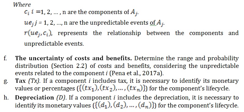
A solution component can incur specific costs (Irani et al., 2006), support materialization of different expected benefits (Irani et al., 2006), be associated with specific economic factors such as taxes and depreciation (Brealey et al., 2011), and be impacted by unpredictable events that imply different uncertainties (Neufville and Scholtes, 2011). Due to these conditions, we can identify the following financial variables at the component level (Pena et al., 2017a).

1. Initial Investment consists of acquisition costs of assets required for a component at time zero (Irani et al., 2006).
2. Benefits are consequences of an action that improve or promote the comfort of a company (Irani et al., 2006) and which are represented as quantified monetary profit in this study (Pena et al., 2017a).
3. Costs consist of the purchase or rental price of a service or asset implied in a solution component (Irani et al., 2006; Smit, 2012) and are represented as a quantified monetary value in this study (Pena et al., 2017a).
4. Economic factors are relevant market and economic data that can influence the value of an IT investment (Irani et al., 2006; Pena et al., 2017a). This study includes taxes, the inflation rate, depreciation, and salvage or rescue value.

Unpredictable Events

Unpredictable events such as changes in providers and new technologies (Vélez Pareja, 2003) create uncertainty levels that must be considered in the variables of the cost-benefit analysis to determine whether the consequences for a company will be positive or adverse (Neufville and Scholtes, 2011; Pena et al., 2017a). An unpredictable event () is defined in consideration of the features proposed by Vélez (Vélez Pareja, 2003) and Neufville (Neufville and Scholtes, 2011): type (economic, technical or regulatory), level of impact (low, medium, high), and variability (low, medium, high).  To measure the uncertainty derived from the , we adopted the activities proposed in the Applied Information Economics model (AIE) (Hubbard, 2010; Mead et al., 2009)[ii] and the definitions of Vélez (Vélez Pareja, 2003).

• Estimating the ranges (low, more probable, very probable) of the cost and benefit variables using expert criteria, subjective probability technique, or historical data (Hubbard, 2010; Vélez Pareja, 2003).
• Quantifying the uncertainty using probability distributions (Cormier, 2010; Hubbard, 2010).

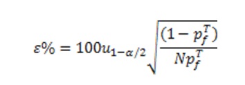
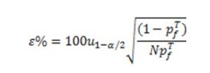
Calculating the error of estimation using Monte Carlo Simulation. This technique depends on the number of samples: the greater the number of samples, the more accurate the estimate will be (Hubbard, 2010; Missouri University of Science and Technology, 2016). If the number of simulations increases, the probability of failure has a lower error in accordance with research done at the University of Missouri (Missouri University of Science and Technology, 2016). Considering that, we use Equation 1 to calculate the error of estimation considering the number of samples N, the probability of failure^pf , and the quartile of standard normal distributions ^.u1-x/2

^[i] High level of granularity refers to estimate values considering alignment with business goals and prioritization of requirements (few details) (Mead et al., 2009), and low-level of granularity refers to decomposition of values in specific variables at the lowest practical level of understanding (Mead et al., 2009).

^[ii] AIE is a rigorous quantitative methodology that presents an explicit method for measuring uncertainty at low levels of granularity and which supports more accurate valuation (Mead et al., 2009).  

Equation 1: calculation of the error of estimation applied to Monte Carlo samples (Missouri University of Science and Technology, 2016)

• Measuring the uncertainty supported by Monte Carlo simulations (Hubbard, 2010).

Other Factors

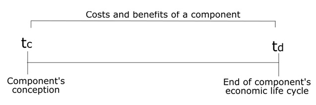
To perform the cost-benefit analysis, the life cycle of a solution component must be considered and therefore costs and benefits must be forecast (Pena et al., 2017a; Smit, 2012). The life cycle comprises activities from conception (t_c) until retirement (t_d) where duration of the lifecycle is given by t_d – t_c (Fig. 2) (Smit, 2012).

Fig. 2:  Component life cycles

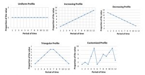
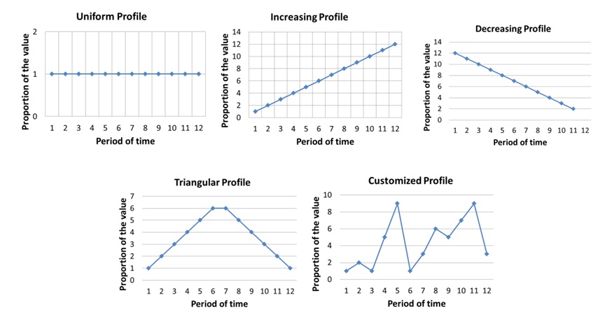
Fig. 3: Examples of profiles 

To determine the cash flows that describe both output flows, the money that a company spends, and input flows, money that a company receives, during the component’s life cycle, we use the five profiles illustrated with examples in Fig. 3. 

Methods of Cost-benefit Analysis

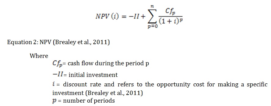
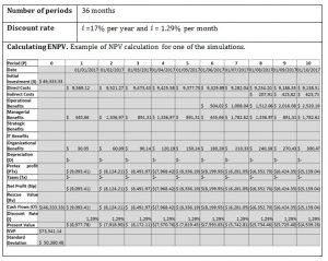
Cost-benefit analysis assesses the effectiveness of budgeted investment as well as the efficiency and profitability of a technology solution (Brealey et al., 2011; Pena et al., 2017a). Cost-benefit analysis is very frequently used to analyze technology solutions (Neufville and Scholtes, 2011; Pena et al., 2017b) and is supported by various methods (Brealey et al., 2011; Mikaelian, 2009; Neufville and Scholtes, 2011). FINFLEX-CBMC uses the Expected Net Present Value (ENPV) method (Mikaelian, 2009; Neufville and Scholtes, 2011) which is an extension Net Present Value (NPV) method (Brealey et al., 2011). NPV (Equation 2) analyzes costs and benefits through accumulation and discounting of cash flows associated with a particular investment (Brealey et al., 2011).

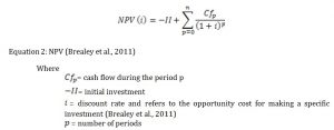
ENPV is used for high-risk projects with unknown levels of uncertainty (Neufville and Scholtes, 2011), and NPV is usually employed on short or certain projects (Neufville and Scholtes, 2011).  While NPV is based on a single forecast of values, ENPV is based on a weighted average according to the probabilities of each of the specific NPVs.  ENPV uses a variable discount rate that reflects the risks of an investment at different points of the time. Finally, unlike NPV which results in a single value (Slot, 2010), ENPV considers a set of NPVs to identify a range of profitability. Therefore, ENPV can consider a greater range of values with greater precision of results (Mikaelian, 2009; Neufville and Scholtes, 2011). We selected ENPV considering the specific characteristics of solution architectures: high-risk investments, long-term returns on investments, high uncertainty levels, and changeable technology environments (Vélez Pareja, 2003).

Related Work

In this subsection, we briefly describe the cost-benefit models we identified, comparisons between and among them, and the objective of this research.

Description of the Cost-Benefit Models Identified

A cost-benefit model is a mathematical representation that comprises one or several equations that are used to analyze how a business reacts to different economic situations and to calculate the outcomes of financial decisions before investments are made (Brealey et al., 2011). We identified the following cost-benefit models in the literature:

Total Value of Opportunity (TVO) is a quantitative and qualitative methodology that seeks to determine the business value of an IT investment (Apfel and Smith, 2003; Cormier, 2010). TVO supports its cost-benefit analysis on Total Cost of Ownership (TCO) (Mead et al., 2009) and supports its uncertainty analysis on the Black-Scholes Option Pricing Model (Apfel and Smith, 2003; Cormier, 2010).

The Cost-benefit Analysis Method (CBAM) has a quantitative approach that guides stakeholders to identify costs and benefits associated with software architecture decisions that result in a system’s quality attributes (Kazman et al., 2002).

Total Economic Impact (TEI) is a model that aims to identify cost supported on TCO, determine the benefit related to the business value and strategic contribution, and analyze uncertainty considering the Black-Scholes model (Cormier, 2010; Mead et al., 2009).

Rapid Economic Justification (REJ) provides a pragmatic expression of the economic justification for an IT investment considering the alignment among its associated costs, benefits, and risks (Mead et al., 2009).   

An Integrated Real Options Framework for Model-based Identification and Valuation of Options under Uncertainty (Mikaelian, 2009) by Mikaelian presents an integrated real options framework (IRF) for holistic analysis of enterprise architecture projects (Mikaelian, 2009). IRF allows the evaluation of enterprise architecture alternatives through modeling of uncertainty, flexibility, benefits, and costs.

A method for valuing Architecture based Business Transformation and measuring the value of Solutions Architecture by Slot (Slot, 2010) presents a method to quantify the values of enterprise architecture that is financially based on business transformation (Slot, 2010). The method considers costs, benefits, and management of uncertainty based on real options (Slot, 2010).

Problems and Objective

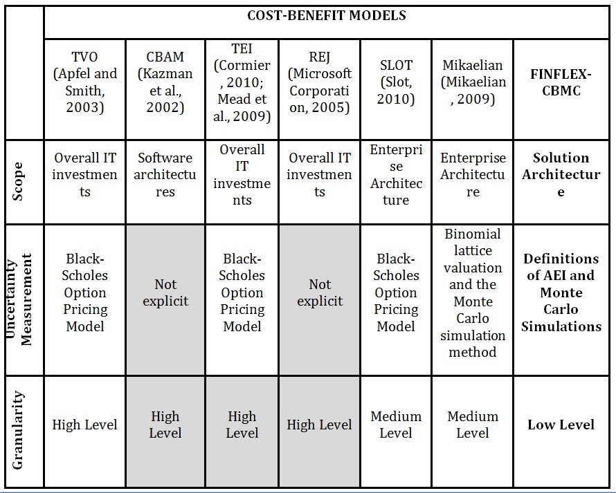
Table 1 compares the cost-benefit models identified.

Table 1: Comparison of Cost-Benefit Models

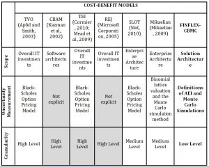
According to the findings presented in Table 1, we identified the following problems:

1. Some of the models are directed to IT overall investments which could restrict the level of detail of the financial analysis of solution architectures needed for considering alternatives and solution components. The models directed toward enterprise architectures have a high level of abstraction and strategic scope that differ from the low level of abstraction of solution architectures and their technological scope.

2. Uncertainty Measurement. To measure uncertainty, some models employ the Black-Scholes Option Pricing Model. According to Hubbard, the Black-Scholes formula is not very clear about how to calculate the price of an option because there is high uncertainty in projections of option prices over time (Hubbard, 2010) while the risk rate is a constant value unlike the variable rates of a solution architecture.

3. Four models have high granularity levels that translate to general financial indicators at the level of IT investments.

Although previous studies offer significant contributions, there is clear evidence that a specific cost-benefit model for analyzing solution architectures had not yet been developed. To respond to these shortcomings, this study aims to define a cost-benefit model addressed to solution architectures that supports financial analysis of alternatives and solution components considering uncertainty.  To achieve our objective, we designed and evaluated FINFLEX-CBMC supported on design science research methodology.

Research Method for Developing and Evaluating FINFLEX-CBMC

We adopted the Design Science Research (DSR) paradigm (Hevner et al., 2004) because it aims to build and evaluate artifacts that solve business needs (Hevner et al., 2004). Our research is valuable to academia and industry because cost-benefit models are valid DSR artifacts (Sonnenberg and Brocke, 2012). FINFLEX-CBMC is supported by the current body of knowledge (Apfel and Smith, 2003)(Kazman et al., 2002) (Cormier, 2010; Mead et al., 2009) (Slot, 2010) and was designed considering the methodology proposed by Avon (Avon, 2013). We followed the DSR evaluation patterns proposed by Sonnenberg and Brocke (Sonnenberg and Brocke, 2012), and we adapted those patterns to FINFLEX-CBMC as shown in Fig. 4. The use of patterns allowed us to demonstrate, design and evaluate FINFLEX-CBMC. We explain below the three evaluation activities used for FINFLEX-CBMC.

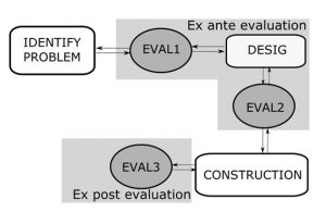
Fig. 4: DSR assesment patterns used for FINFLEX-CBMC. Adapted from (Sonnenberg and Brocke, 2012)

1. Identifying problem and objectives of FINFLEX-CBMC. The first evaluation (EVAL1) justified the research problem and supported its contribution to both industry and literature. EVAL1 was completed in Sections 1, 2, and 3.

2. Designing FINFLEX-CBMC. The second evaluation (EVAL2) justified the design of FINFLEX-CBMC (Sonnenberg and Brocke, 2012). We designed FINFLEX-CBMC by adopting definitions from the financial model of design proposed by Avon (Avon, 2013). We considered the following assumptions in the design of FINFLEX-CBMC  (Avon, 2013):

1. Alternatives and their components respond to the business or technology requirements that inspired them.
2. Alternatives and their components are technically equivalents and have been technically analyzed by a company.
3. Financial variables and economic factors of a solution component have been identified and estimated through methods previously selected by

3. Constructing FINFLEX-CBMC. The third evaluation (EVAL3) justified the utility of FINFLEX-CBMC (Section 6). To execute EVAL3, we first defined the cost-benefit model (Sections 5). Then, we created a prototype of FINFLEX-CBMC to capture the required data, perform the cost-benefit analysis and present the results (Section 6).

An Innovative Cost-Benefit Model for Analyzing Solution Architectures Considering Uncertainty

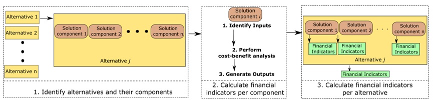
To describe FINFLEX-CBMC, we used the generic process presented in Fig. 5. It includes the essential activities required for calculating the financial indicators of an alternative and its solution components.

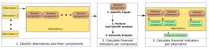
Fig. 5:  Generic Process of FINFLEX-CBMC

Identifying the alternatives and their components

This activity defines the solution architecture alternatives of a technology solution and identifies the solution components of an alternative.

Calculating the financial indicators by component

The process considers the activities explained below in order to calculate the financial indicators of a component.

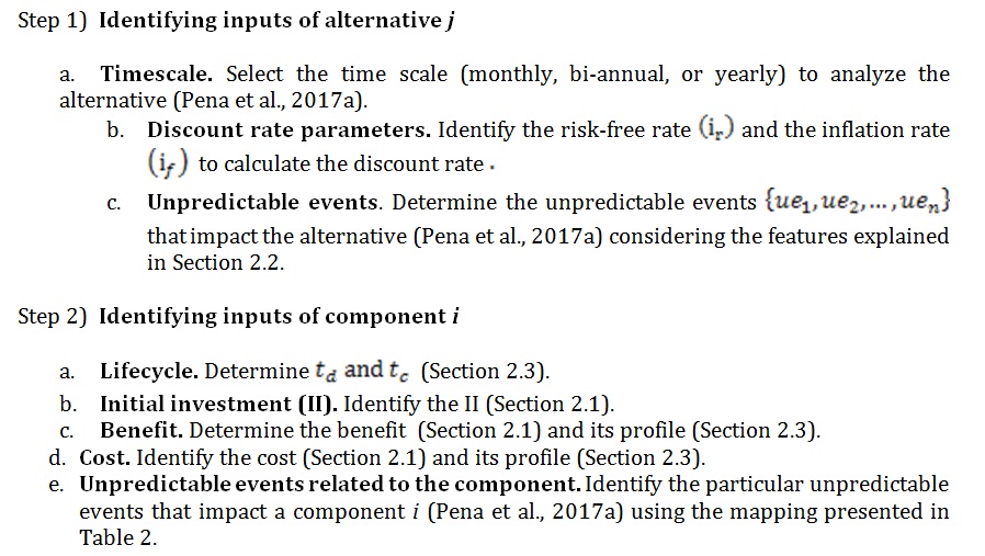
Identifying inputs 

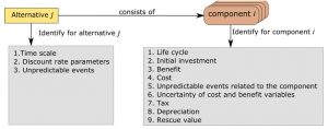
Fig. 6: Inputs required for FINFLEX-CBMC 

As Fig. 6 presents, inputs have two sources: alternatives and components. The alternatives’ inputs are used to perform the cost-benefit analysis for all of the alternatives’ components while the components’ inputs are particular to each component. 

Input identification considers two steps:

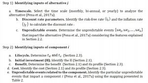
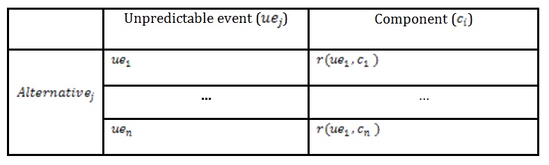
Table 2 : Mapping between alternatives’ unpredictable events and components

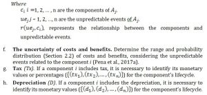
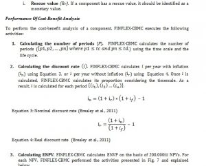
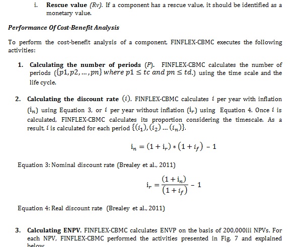
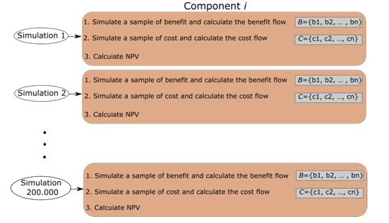
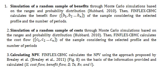
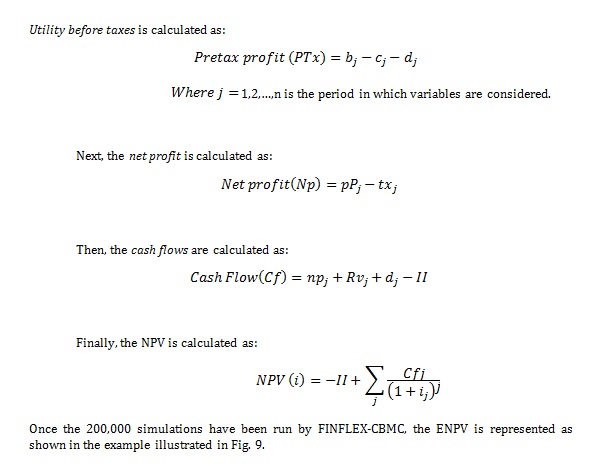
Fig. 7: ENPV calculation using Monte Carlo simulations

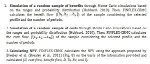
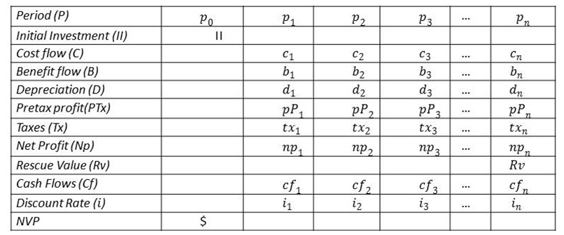
Fig. 8:  Approach to calculation of NPV (Brealey et al., 2011)

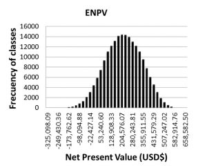
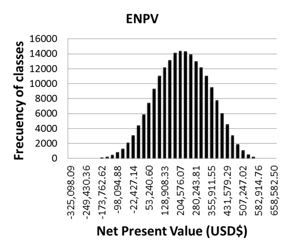
Fig. 9: Example of ENPV

Generating outputs

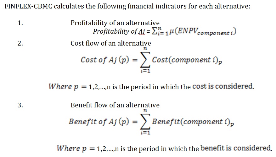
FINFLEX-CBMC generates the following financial indicators for any component :  

     1. ENPV

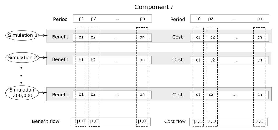
2. Benefit flow and cost flow as shown in 10. The benefit and cost flows are identified by calculating the mean (µ) and standard deviation (σ) of the simulated variables for each period.

3. Cash flow.

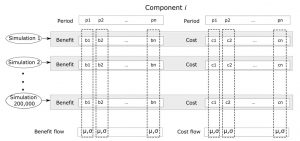
Fig. 10:  Calculation of the cost and benefit flows of a component

Calculating the financial indicators for each alternative

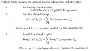
Fig. 11 presents the results of the financial indicators at the component and alternative levels as calculated by FINFLEX-CBMC. This result supports the comparison between components and alternatives and provides detailed data to support investment decisions.

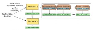
Fig. 11:  Financial indicators at alternative and component levels

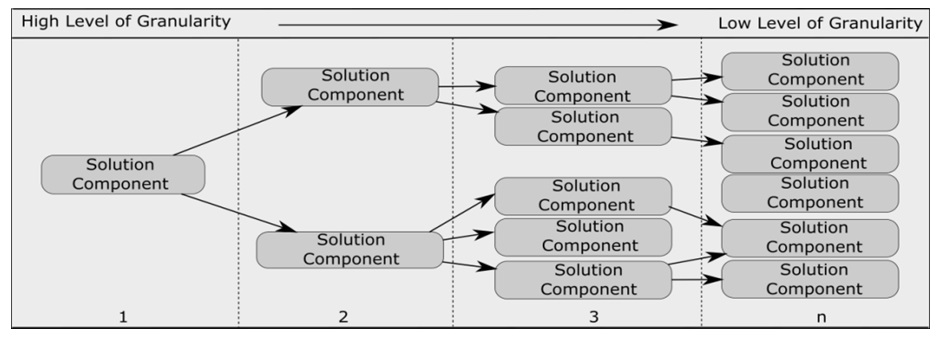
Finally, as Fig. 12 shows, the design of alternatives is commonly an iterative process in which the first iteration has a high level of granularity and the last iteration has a low level of granularity.  FINFLEX-CBMC can be used independently of the alternative’s granularity. 

Fig. 12: Level of Granularity of alternatives

Evaluation of FINFLEX-CBMC

FINFLEX-CBMC was evaluated to justify its utility based on the scenarios method (Hevner et al., 2004). This method was selected because we evaluated FINFLEX-CBMC on the basis of six scenarios that were performed by 32 IT professionals distributed into six teams. EVAL3 was conducted between August 2016 and December 2016 as part of the Solution Architecture course offered by the master’s degree in Architecture of Information Technology of Los Andes University (https://sistemas.uniandes.edu.co/en/mati-en). Each scenario represented between one and three solution architecture alternatives that responded to the requirements of a hypothetical company called CCT. CCT offers technology services based on Business Process Outsourcing within Colombia and internationally. CCT currently has difficulty managing customer data related to information traceability and consolidation. Consequent high levels of customer dissatisfaction have increased risks of losing customers and sales opportunities. Appendix A presents an example of one alternative defined by one of the teams.

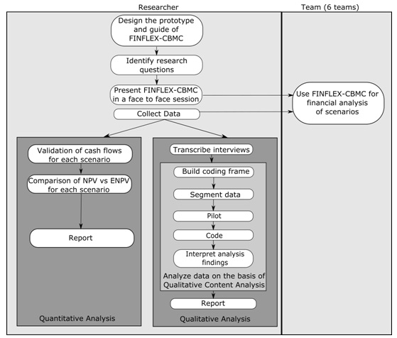
The evaluation methodology is presented in Fig. 13. Due to space limitation, we have only briefly described the quantitative analysis. As Fig. 13 shows, we first designed a prototype and a guide for FINFLEX-CBMC. Then, we identified research questions to determine how FINFLEX-CBMC supports financial analysis of solution architectures. Next, we presented the prototype and the guide to the six teams in a face-to-face session. Subsequently, the teams evaluated their alternatives using FINFLEX-CBMC. Finally, we collected and analyzed the instances of the prototype with scenarios defined by the teams (A total of 12 solution architecture alternatives because some of the teams only defined one alternative for each scenario).

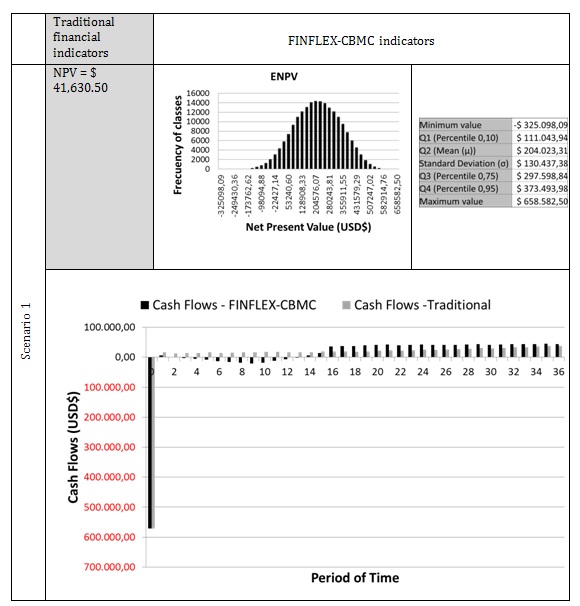
The objective of the quantitative analysis was to compare traditional financial indicators with the financial indicators generated by FINFLEX-CBMC. Specifically, we compared NPV and ENPV and the cash flows of these approaches. Table 3 presents the results of the financial indicators of one example for three alternatives that had a high level of granularity. For this reason, each alternative was analyzed as a unique component.

Fig. 13: Methodology for evaluating FINFLEX-CBMC 

Table 3: Scenarios considered in quantitative analysis  

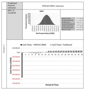
It can be seen from the results that, while the NPV offers a unique value for identification of the profitability of a solution, the ENPV is a rich source of data for analyzing risks and possibilities of profitability.

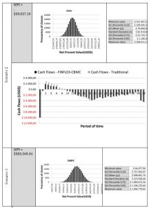
For example, in scenario 1, the NPV is $ 41,630.50 which could be a good basis for making a decision since it is positive. However, the NPV’s value is lower than the mean (μ) of ENPV which is $204,031.30 and, since the standard deviation (σ) of ENPV is $130,437.38, profitability is likely to be nearly 50% higher than that indicated by NPV alone. ENPV can give experts more information for each percentile plus the standard deviation measures possible risks of an investment. It is also interesting to analyze the minimum and maximum profits of a solution. For example in scenario 2, the minimum profit is -$322.467, the maximum profit is $298.911, and the average profit is -$70.840. In this scenario, experts can identify the maximum and minimum possible profits as well as the risks thereby providing more robust information to support investment decisions.

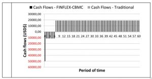
The scenarios reveal some differences regarding cash flows between the traditional NPV and the ENPV which could affect the identification of outflows and inflows that in turn could result in notable differences regarding investment in a particular solution. The ENPV’s cash flows are the results of simulations which may provide more certainty to the analysis.

Finally, on the basis of the results of the quantitative evaluation, we concluded that FINFLEX-CBMC offers more detailed and richer financial indicators than does the traditional NPV for making investment decisions regarding solution architectures. 

Discussion and Future Work

This paper has presented FINFLEX-CBMC, a cost-benefit model that calculates financial indicators of solution architectures on the basis of their components and alternatives. FINFLEX-CBMC contributes to the determination of unpredictable events and measurement of uncertainties to determine positive and adverse events related to an investment.  FINFLEX-CBMC has a number of advantages:

• It calculates financial indicators at two levels of detail for solution architectures: alternatives and components.
• It permits comparison of financial indicators for components and alternatives and measures uncertainty associated with financial variables which can increase the accuracy of the indicators calculated.
• It consolidates financial variables and financial indicators related to solution architectures. FINFLEX-CBMC’s flexibility allows performance of sensitivity analysis on the basis of the variation of the financial variables, and it supports risk analysis of IT investments on the basis of ENPV and its metrics.

Although FINFLEX-CBMC provides a complete set of calculations and supports a cost-benefit analysis of solution architectures, it does have some limitations. These include the amount of data required for the use of FINFLEX-CBMC,  the performance of the FINFLEX-CBM’s prototype, and absence of the experience of the architects in the interpretation of financial indicators of stochastic models like FINFLEX-CBMC. Consequently, results could be omitted or misunderstood by an interdisciplinary team.

We are considering the following activities to continue the development of FINFLEX-CBMC:

1. Implementation of the prototype on another platform that improves performance and user experience.
2. Definition of a methodology to support FINFLEX-CBMC that will offset the absence of experience interpreting financial indicators. We propose to include detailed examples and descriptions to identify the utility of the financial indicators.
3. Validation of FINFLEX-CBMC with case studies to provide more details and use of the model in real cases.
4. Analysis of historical data to support FINFLEX-CBMC and to reduce the complexity of the analysis.

Acknowledgements

The authors of this paper would like to thank the group of professionals of the Master’s Degree of Architecture of Information Technologies at Los Andes University for participating in the evaluation of FINFLEX-CBMC. Their comments and scenarios have helped us identify the advantages and disadvantages of our financial model, as well as pointing towards future research to improve our work.

References

1. Apfel, A. and Smith, M. (2003), TVO Methodology: Valuing IT Investments via the Gartner Business Performance Framework, Strategic Analysis Report, Gartner, USA, available at: https://www.gartner.com/doc/387459/tvo-methodology-valuing-it-investments (accessed 25 September 2016).

2. Arango Serna, M.D., Londoño Salazar, J.E. and Branch Bedoya, J.W. (2015), “Solution architecture approach, mechanism to reduce the gap between enterprise architecture and implementation of technological solutions”, Dyna, Vol. 82 No. 193, pp. 117–126.

3. Avon, J. (2013), The Handbook of Financial Modeling, 1st ed., Apress, New York, NY, available at:https://doi.org/10.1007/978-1-4302-6206-0.

4. Brealey, R.A., Myers, S.C. and Allen, F. (2011), Principles of Corporate Finance, edited by Mcgraw Hill Book Co, 10th ed., McGraw-Hill/Irwin, New York, USA.

5. Cormier, B. (2010), The Total Economic Impact Of Cisco ’ S Borderless Networks, Forrester, Cambridge, MA, USA, available at: http://www-test.cisco.com/c/dam/en/us/solutions/collateral/routers/3900-series-integrated-services-routers-isr/bn_TEIstudy.pdf (accessed 16 June 2015).

6. Hevner, B.A.R., March, S.T., Park, J. and Ram, S. (2004), “Design Science in Information Systems Research”, MIS Quarterly, Vol. 28 No. 1, pp. 75–105.

7. Hubbard, D.W. (2010), How to Measure Anything Finding the Value Of “intangibles” in Business, 2nd ed., John Wiley & Sons, New Jersey, U.S.

8. Irani, Z., Ghoneim, A. and Love, P.E.D. (2006), “Evaluating cost taxonomies for information systems management”, European Journal of Operational Research, Vol. 173 No. 3, pp. 1103–1122.

9. Kazman, R., Asundi, J. and Klein, M. (2002), Design Decisions : An Economic Approach, Pittsburgh, PA, available at: http://resources.sei.cmu.edu/library/asset-view.cfm?AssetID=6265 (accessed 20 January 2016).

10. Mead, N., Allen, J.H., Conklin, W.A., Drommi, A., Harrison, J., Ingalsbe, J., Rainey, J., et al. (2009), Making the Business Case for Software Assurance, SPECIAL REPORT CMU/SEI-2009-SR-001, Pittsburgh, PA, available at: http://resources.sei.cmu.edu/library/asset-view.cfm?assetid=8831.

11. Microsoft Corporation. (2005), Rapid Economic Justification, A Step-by-Step Guide to Optimizing IT Investments That Forge Alliances Between IT and Business, Microsoft, WA, USA, available at: http://mbstrauch.com/wp-content/uploads/2013/03/Book_MSFT_REJ_Enterprise_.pdf.

12. Mikaelian, T. (2009), An Integrated Real Options Framework for Model-Based Identification and Valuation of Options under Uncertainty, Massachusetts Institute of Technology, available at: http://hdl.handle.net/1721.1/51676.

13. Missouri University of Science and Technology. (2016), “Monte Carlo Simulation”, Probabilistic Engineering Design, Missouri University of Science and Technology, Columbia, USA.

14. Neufville, R. De and Scholtes, S. (2011), Flexibility in Engineering Design, MIT., Massachusetts Institute of Technology, London, England.

15. Pena, Y., Correal, D. and Miranda, E. (2017a), “FINFLEX-CM: A conceptual model for financial analysis of solution architectures considering the uncertainty and flexibility”, edited by Solano, A. and Ordóñez, H.Communications in Computer and Information Science, Springer International Publishing, Cali, Colombia, Vol. 735, pp. 242–256.

16. Pena, Y., Correal, D. and Miranda, E. (2017b), “A review of the current situation, challenges and opportunities in the financial analysis of enterprise architectures”, World Review of Science, Technology and Sustainable Development (WRSTSD), Vol. 13 No. 2, pp. 145–173.

17. Slot, R. (2010), A Method for Valuing Enterprise Architecture Based Business Transformation and Measuring the Value of Solutions Architecture, University of Amsterdam, available at: http://dare.uva.nl/document/2/72277.
18. Smit, M. (2012), “A North Atlantic Treaty Organisation framework for life cycle costing”, International Journal of Computer Integrated Manufacturing, Vol. 25 No. May, pp. 444–456.

19. Sonnenberg, C. and Brocke, J. (2012), “Evaluations in the Science of the Artificial – Reconsidering the Build-Evaluate Pattern in Design Science Research”, in Peffers, K., and Rothenberger, M. and and Kuechler, B. (Eds.), Proceedings of the 7th International Conference on Design Science Research in Information Systems: Advances in Theory and Practice, Springer-Verlag, Las Vegas, NV, pp. 381–397.

20. Vélez Pareja, I. (2003), “Decisiones bajo incertidumbre”, in Norma, G.E. (Ed.), Decisiones Empresariales Bajo Riesgo E Incertidumbre, Grupo Editorial Norma, Bogotá, Colombia, p. 48.

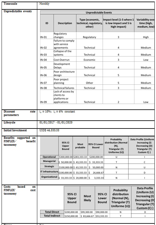
Appendix A – Example of the use of FINFLEX-CBMC

This case presents a proposal by team one for an integrated solution to meet CCT’s requirements which is supported by the Oracle platform. This alternative had a high level of granularity, so it was analyzed as a unique component.

Identifying Inputs

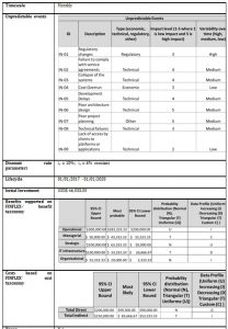
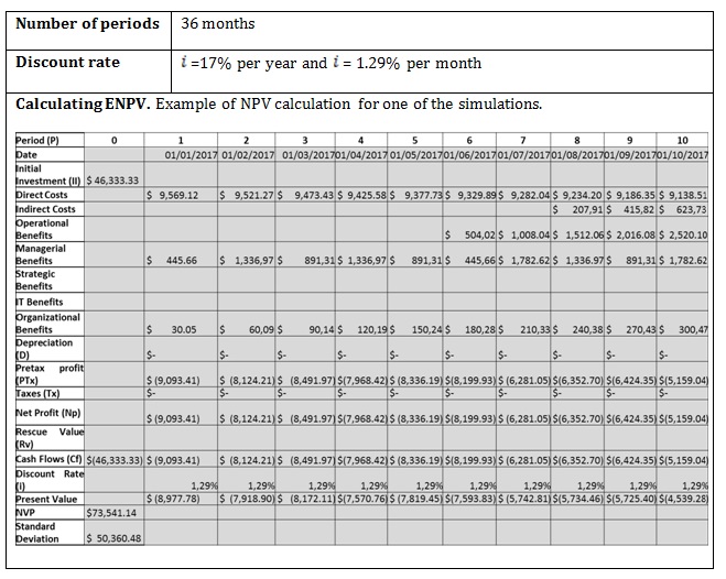
Performing cost-benefit analysis

1. Generating outputs

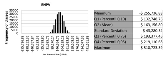
1. ENPV (Fig. 14)
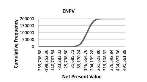
2. ENPV – cumulative frequency ( Fig.15)
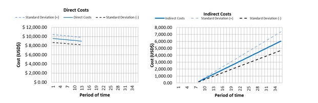
3. Cost flows ( Fig.16)
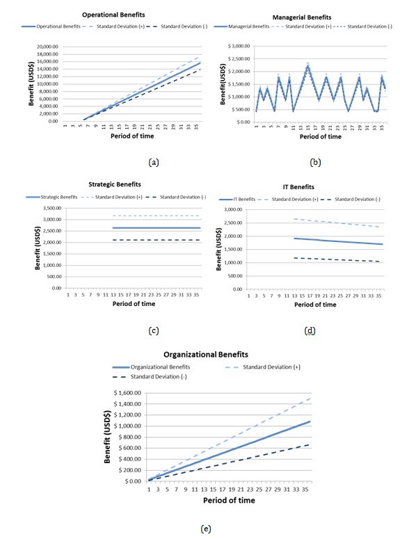
4. Benefit flows ( Fig.17 )
5. Cash flows ( Fig.18)

Fig. 14: ENPV of alternative 1

Fig. 15: ENPV of alternative 1 – cumulative frequency 

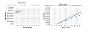
Fig. 16:  Costs flow with standard deviation of alternative 1 

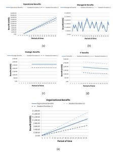
Fig. 17:  Benefits flow with standard deviation of alternative 1  

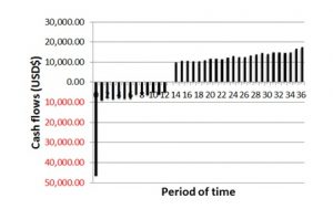
Fig. 18: Cash flows of alternative 1