Hajar ABOUS, Mhamed HAMICHE and Mohamed El MEROUANI
University of Abdelmalek Essaâdi-Morocco
Volume 2020,
Article ID 359922,
IBIMA Business Review,
14 pages,
DOI: 10.5171/2020.359922
Received date: 20 April 2020; Accepted date: 28 May 2020; Published date: 28 July 2020
Cite this Article as:
Hajar ABOUS, Mhamed HAMICHE and Mohamed El MEROUANI (2020)," Optimization of Transshipment Operations: Simulation of the APM Terminal/Tanger Med Port Case ", IBIMA Business Review, Vol. 2020 (2020), Article ID 359922, DOI: 10.5171/2020.359922
Container terminals, which are part of the global port system, represent important hubs of this intermodal transport system. Therefore, the need to improve operational efficiency is the most important problem for container terminals from an economic point of view. In this article, the main objective is to simulate a transshipment operation in the port of Tangier. A mathematical model is developed to formulate an integrated processing system and find an efficient solution algorithm for the Rubber-tyred gantry (RTGs) deployment as a handling equipment for container stacking at terminals, taking into account both the loading and unloading times. This model takes into account the loading and unloading operations time as well as quay crane and yard crane (Y.C). This model’s goal is to constitute a cost reduction strategy. By reducing this transshipment equipment use, this model takes into account the specific objective of minimum total cost, including both the optimal RTGs usage and the total operations time for the quay cranes (QC)
Containerized sea freight transport is a preferred mode of transport, because the use of containers reduces the amount of packaging and product damage. Operational research methods have been widely used to optimize the performance of container terminals, measured by parameters such as the waiting time of ships at docks, the length of time containers stay at the terminal and the degree of congestion due to heavy container handling operations. The management of container terminals faces five typical problems: allocation of berths, planning of quay cranes, sorting operations, transfer operations and planning of mooring and stowage of vessels. One of the most important processes of a container terminal is the streamlining of incoming and outgoing (import / export) flows of containers. The goal of these operations is to maximize the operational productivity by efficiently using space for storage as well as the use of QC, YC and RTG handling equipment. The import/export containers processes are divided into several sub-blocks; each one is made up of a certain number of rows. A storage area is made up of several stacks of a certain size (levels) and can contain both 20 ’and 40’ containers.
These trips are costly for a container terminal and must be minimized. Inefficient storage plans and management can cause bottlenecks or operational delays in container flows. There are many logistical studies in the container storage literature on different aspects. Agostino et al (2019) have developed a simulation model of operations in the train arrival process at Port Terminal of Ponta da Madeira, aiming to develop a simulation model to support decision making. Their study verified that the developed model presented adherence to actual behavior of the system studied, being valid for the operationalization, as a tool to support decision making. Guedj et al. (2007) considered that the container terminal at the port of Koper, in Slovenia, used a Petri net and a genetic algorithm to manage the problems of berthing and loading/unloading of the containers. Lee and Kim (2013) studied the optimal layout of container parks, taking into account the storage space requirements and the throughput capacities of cranes and transporters. Most of the published studies have used simulation to model container storage operations. The paper of Carboni and Deflorio (2020) presents a micro-simulation approach for evaluating the flexibility of typical railroad terminals in a critical scenario, such as the temporary inaccessibility of a gantry crane. The proposed simulation method is not only used for performing a typical sensitivity analysis under troubled conditions, but also for assessing the flexibility of the simulated terminal. To compare the modeled scenarios, some quantitative key performance indicators (KPIs) are designated and quantified in terms of quality and energy impacts.
Several other studies include analysis and optimization models. Sauri and Martin (2011) described three stacking strategies to improve site performance. The metric variables used were the time spent in the storage area. Soriguera et al. (2006) analyzed the internal transport subsystem of a shipping container terminal and examined the effect of the type of handling equipment used in Barcelona container terminal.
Preston and Kozan (2001) studied modeling and determining the optimal storage strategy for various container handling schedules. The problem was formulated and solved by a genetic algorithm in order to minimize the container’s transfer times. Lee et al. (2009) studied the integrated problem of bay distribution and the problem of planning sorting cranes for transshipment containers. However, Chen and Lu (2012) considered an allocation problem for export containers. The goal was to maintain the stability of the vessel and minimize the handling efforts of the dock cranes and yard equipment.
In this scientific studies context, this paper will rather focus on optimizing the time and costs of handling operations within a terminal related to the company APM TERMINAL which is an active transshipment operator within the Tangier MED port. It manages and operates one of the most important container terminals in Morocco. This port is located in the far north of the country overlooking the Strait of Gibraltar at the crossroads of maritime traffic. Due to its strategic location in the Mediterranean Sea, the port is an ideal node for import / export between Europe, Asia and Africa.
The basic idea of modeling and objective function
Based on practical experience, the cost of docking vessels is generally higher than the cost of operating fishing vessels. Therefore, in this paper, the first principle is that the mooring time of the unloading vessel should be as short as possible. To this end, it is necessary to ensure that there are sufficient RTGs for the loading and unloading operations to take place without stopping. The time during which an RTG completes an unloading and loading cycle is random and also depends on the distance of the path traveled, as well as the unloading and loading position chosen an RTG. The aim of this paper is to find all the different paths and to strategically choose the longest one as the basis for decision.
Assumptions and problem analysis
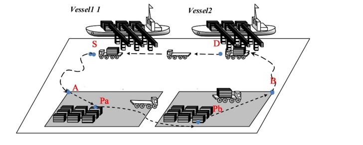
This paper will help RTGs reach full employment. RTGs work on the path between QCs and storage areas and other empty RTGs can be dynamically added to the current line at any time. It can reduce the waiting time for RTGs and make full use of the cranes. The QC costs of unloading at the berth are taken into account, as well as the costs of the RTGs. The combination of operations is illustrated in Fig 1.
Fig. 1: A cycle of RTG travel routes
Modelization
This problem will be developed in the form of a mathematical model with constraints and an objective function, as well as certain problems which can also be described in the form of mathematical formulas, which are used to replicate and define the simulation.
Ratings and Variables
The data sets, variables and parameters used in the formulation are defined before developing the mathematical model.
The data:
R : Total travel distances,r ∈ R
N – : Total number of containers to be unloaded,
N+: Total number of containers to be loaded c,c’ ∈ N+
A : The storage points defined in the storage yard are determined to handle the unloading containers, a ∈ A
B: The storage points defined in the storage yard relate to the handling of containers for loading the ship, b ∈ B
I: Total number of RTGs
L: Total number of cycles performed by all RTGs
Index:
r: Index of the different travel distances, r = 1,…, R
a: Index of points in zone S1 used for storage, a = 1, …, A.
b: Index of points in zone S2 of containers intended for ships, b = 1, …, B.
c: Index of containers to be loaded, c = 1,…,N+
i: Index of the different RTGs, i = 1,…, I
l: Index of the different cycles carried out by each RTG, l = 1, …, L.
Variables:
k: The number of RTGs used
Pa: The random position in the yard S1 available for storage Pa (xa, ya) S1
Pb: The position available in the yard for loading on the ship Pb = (xb, yb) S2
MC (k) : Cost of unloading QC with k RTG.
dr: Distance traveled by the rth course, r ≥ 6
dil: The distance from the Pth cycle of the ith RTG
oil: The number of loading containers
til: Working time of the Pth cycle of the ith RTG
Settings:
Qut0 : The time in minutes of an unloading operation with a QC (min)
Qlt0 : The time in minutes of a loading operation with a QC (min)
d1: Distance between the unloading vessel and the storage yard S1 (S → A)
d2 : Distance between the loading storage yard and the loading vessel (B → D)
d3: Distance between the two vessels (D → S)
R ut0: The duration of an RTG operation in the storage yard (S1) (min)
R lt0 : Duration of an RTG operation in the loading yard (S2) to the ship (min)
V/rtg : The speed of an RTG (meter / minute)
MC0: The unit cost of unloading QC ($ / min)
V C0: Unit cost for an RTG ($ / min)
m1, m2, n1, n2: Length and width of the two storage areas (S1, S2).
Mathematical analysis and objective function
(1) According to the first principle, in order for the docking time of the unloading vessel to be as short as possible, it is necessary to assign a sufficient number of RTGs to the point of unloading for the system to operate without stopping. Thus, from this moment, there should be at least one RTG in each time unit of QC operation.
k = maxiltil/Qut0 is used to calculate the number of RTGs required, and the maximum time value for all the cycles is obtained by selecting the longest cycle distance that would occur in each simulation.
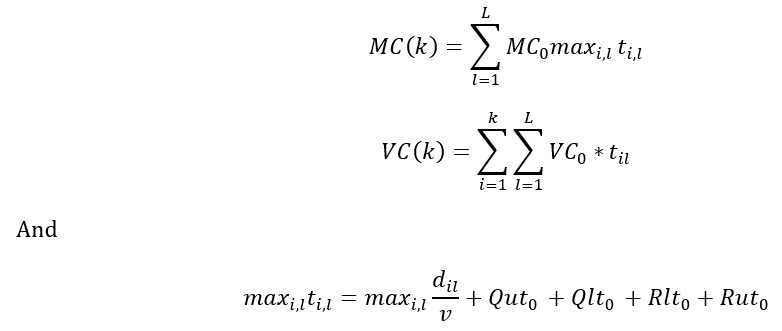
(2) As indicated in the hypotheses and the analysis of the problem, two cost elements are taken into account in the objective function: QC handling operations, the cost of the ship in unloading situation and the cost of using the RTG.
Therefore, the objective function of this integrated processing system model based solely on RTG planning could be expressed as follows:
Based on the previous analysis, the objective of this problem is to minimize the total cost of this integrated operation, which is indicated as follows:
To define specific cost functions,
Constraints
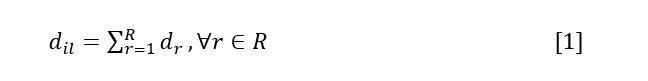
(1) Distance constraints: For the total distance traveled by an RTG, the equation is given as follows:
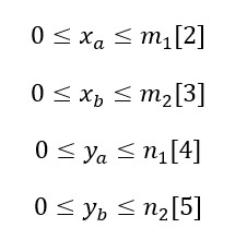
(2) The constraints of the storage area (yard): Equations [2] and [5] show the coordinates of the storage areas in order to define the size of the yards.
(3) Container and loading sequence constraints: To simplify the model and make RTGs efficient, each incoming container is associated with an outgoing container. This means that the unloading and loading volumes are balanced. Equation [6] illustrates this relationship:
As previously stated, there should be a rule for the sequence of loading containers onto ships from the shipyard. To take this point into account and facilitate the development of the model, the containers are defined in four groups with different values and the collection sequence of the containers is to be loaded according to the aforementioned value. Containers with the highest number will be loaded first. As in equation [7], the value of container c + 1, which is the next container to be loaded, immediately following container c, will be loaded in the place of loading and cannot be exceeded by the value of the last container which has just been loaded. It should be a certain rule in which the smallest number of containers cannot come before a larger number of containers.
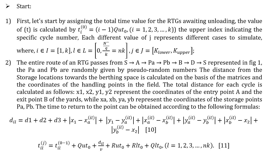
The purpose of this model is to search in the simulation for the best number of RTGs at the lowest cost. The object of the simulation is therefore to find the optimal number of RTGs. The total duration of an RTG cycle includes the journey time of the six sections and the time of the RTG of loading and unloading operations in these two sites (S1, S2), as well as a loading and unloading operation of the CQ, which is formulated in the following equation:
The equation neglects the QC operation time of the loading vessel because the cost of QC at the berth in the objective function is concentrated on this vessel being unloaded. RTG operations are optimized only for this vessel. In addition, according to the total time per cycle, the number of RTGs is very important, which must be used to meet the volume requirement to load or unload without waiting time for QC, so that handling operations of QC do not stop. The value calculated by the equation below can reach a zero-time interval in each cycle (no waiting) to make the operations continuous and successive:
Since the duration of each RTG cycle varies according to the reach of the different storage points, there is a maximum value , among all the possible results. The unloading operations will never stop in case of .The Monte Carlo method is a calculation method leading to approach optimal solutions by probability statistics.
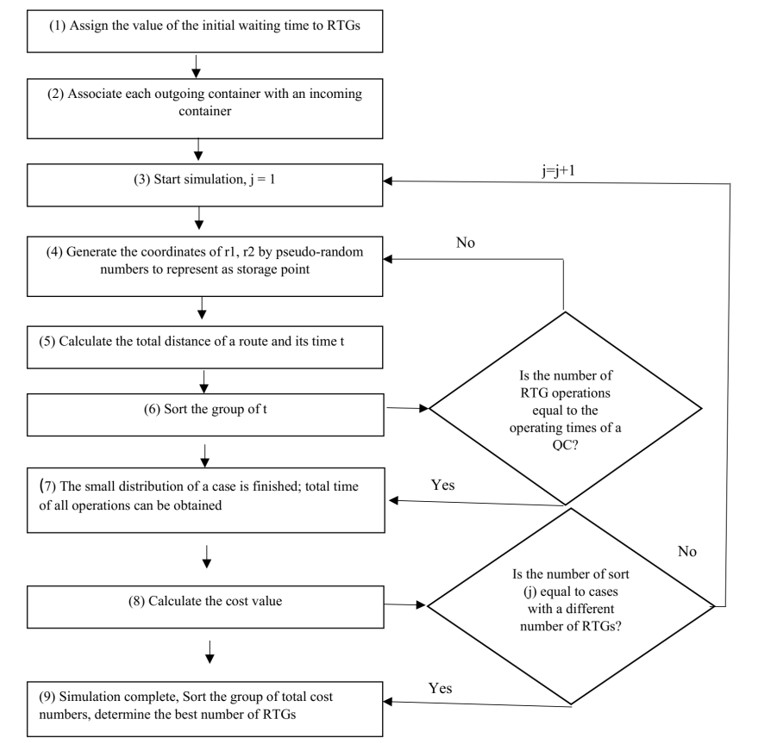
As a premium on board, in this model, this method is proposed to generate pseudo-random numbers for the points in the storage fleet. The objective is to be able to represent the actual storage position of the containers in the simulation. The yards will be expressed in the form of matrices and each storage point will be noted 0 or 1 to define the condition of each storage location. Thus, in this paper, the different models with different RTG numbers will be simulated on an experimental basis. This will be the main objective of this simulation. In particular, the steps of the algorithm developed for this specific problem are expressed in the logical flow diagram. (See fig. 2).
Fig. 2: Flowchart of the algorithm
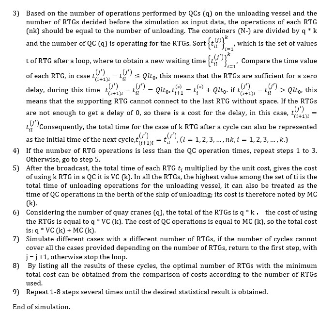
On this basis, the specific steps and the corresponding calculation methods are introduced in the following elements:
Results
Based on real data, the values of the parameters and the scenarios of all the probabilistic cases can be defined by means of a computer simulation.
Test Design and Results
There are two ships docked at one time. They must be unloaded and loaded simultaneously. The total number of unloading operations from the ship is 2400. To balance the movements of the RTGs, the loading volume is also 2400.The containers considered in this model are equivalent units to twenty- and forty-foot containers. Each RTG has a total loading capacity of two twenty-foot containers or a single one of forty feet. to facilitate the simulation, the total loads will be calculated as following:
In addition, the distance between the unloading ship and the shipyard S1 is 1 km, the distance between the other shipyard S2 and the loading ship is 1 km and the distance between these two ships is 300 km. The unit time for QC is 5 minutes per load movement, for both loading and unloading operations. The unit time for RTG unloading operations is 6 minutes per container. However, the unit duration of RTG loading operations is 6 minutes per charge. The speed of RTG is 20 km/hour. The unit cost of using the RTGs is assumed to be $ 1/minute, and the unit cost of QC at the berth of the unloading vessel is $ 5/minute. The spatial positions of the containers in the storage areas are generated randomly by matrices via MATLAB. These two stocks S1, S2 are represented by two-dimensional coordinate matrices (abscissa and ordinate), in order to calculate the distances. The height of the sub-block is considered authorized in construction sites in 4 levels. Each coordinate linked to a container can correspond to a number between 1 and 4 to indicate its location while showing the number of containers already present in this point.
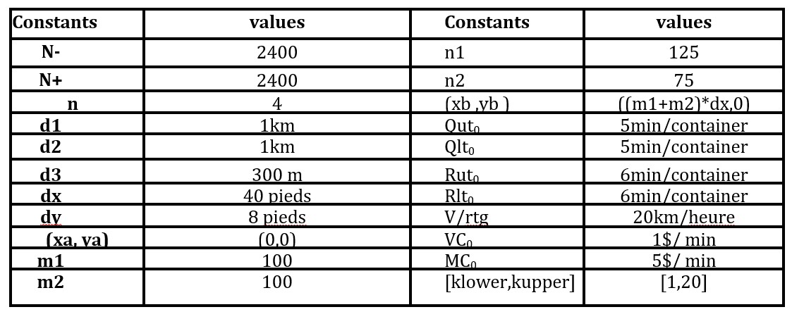
To examine the loading sequence of these containers in S2 in the ship, they are separated into four groups, with a different number to represent the situation of the containers in each group: 4,3,2,1: the containers classified in group 4 must be loaded first, then 3, 2, 1. The containers with the smallest numbers cannot be loaded first if there is still a group of containers with a larger number, according to this model’s hypothesis. In practice, the loading operating mode follows the rules of this design. As this model does not consider loading details, the loading sequence is simplified with notation numbers; therefore, other aspects such as weight, destination, etc. … are not taken into account. It is assumed that there are six sections to compose the total distance of the circuit of an RTG. The distances of the sections are located in building sites S1 and S2. They would be calculated according to the coordinates (abscissa X, ordinate Y). As the calculation of the distance is a carried out based on the site plan, therefore the x, y coordinates of each point are needed. It us also assumed that the capacity of site S1 in the model is 100 * 75 * 4 (length * width * height), which makes a total storage capacity of 30,000 units, while S2 corresponds to 100 * 125 * 4, with a total capacity of 50,000 units. Thus, two matrices having values of 0 or 1, are generated by MATLAB. The first matrix (S1) having the mentions 100 * 75 (length * width), the second (S2) is 100 * 125, the space of each point is defined by the size of the containers, the horizontal space is 40 feet and the longitudinal space is 8 feet. Before the simulation and on the basis of the hypotheses mentioned above, the constant input data is shown in the following table.
Table 1: Input data
Since the storage points in the construction sites are generated randomly in this model, the distance of the route is variable from different simulations. To validate the results and the models, 10,000 simulations are repeated to obtain the statistical results. After 10 000 simulations executed in MATLAB, the results with these specific inputs are presented in table 1 The figures show the cost function.
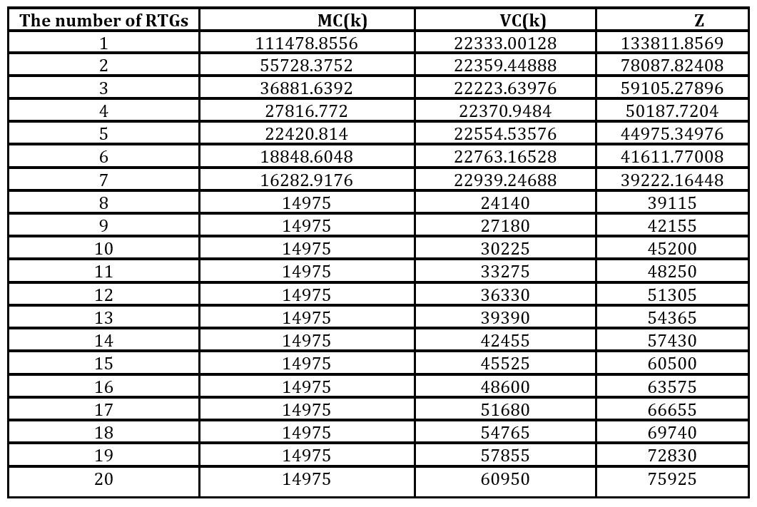
Table 2: Average value of 10,000 simulations performed
The cost of the RTGs used for each QC increases gradually depending on the number of RTGs used. Indeed, after having tested 8 RTGs; the cost of docking in the unloading station has a typical characteristic: in cases where 1 to 8 RTGs are affected; the value decreases when the number of RTGs increases, while the service time decreases. However, in the case of 8 RTGs, this cost function is convergent, as shown in the following figures (3, 4, 5 and 6).
Fig. 3: Results of scenario 1: cost of the RTG in use for each QC: VC (k)
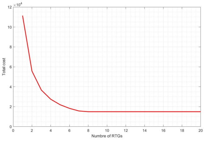
Fig. 4: Results of scenario 1: cost From QC to the quay of the unloading vessel: MC (k)
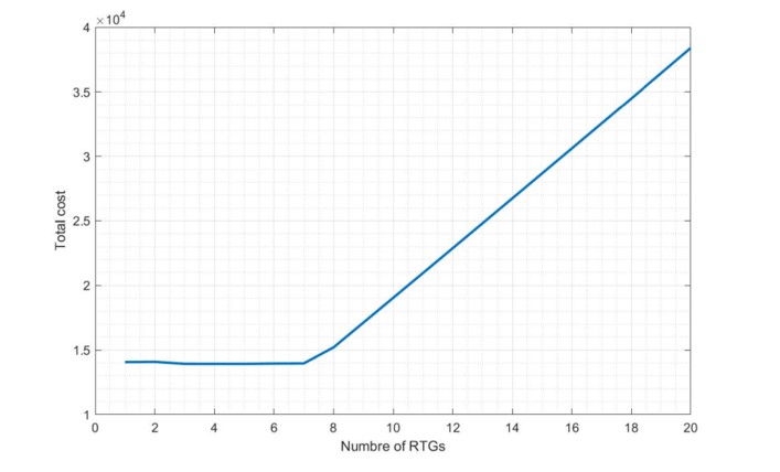
Fig. 5: Results of scenario 1: total cost: Z
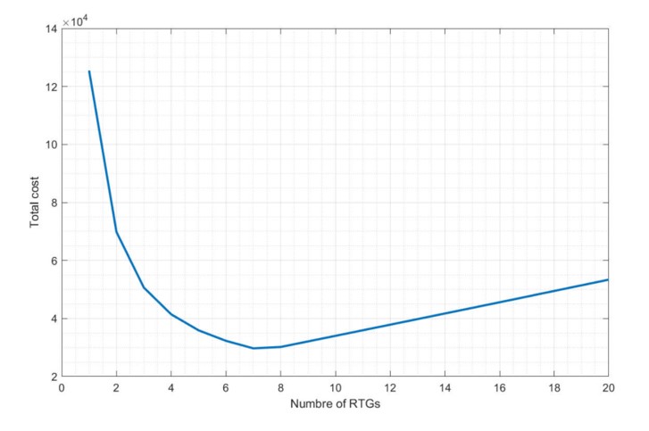
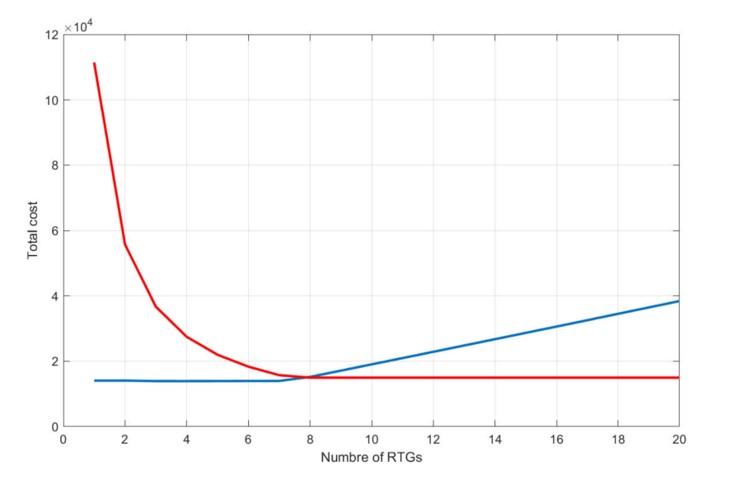
Fig. 6: Results of scenario 1: break-even point for the optimal number of RTGs
From the results obtained, the cost of QC in the unloading station is constant; this means that the 8 RTGs are sufficient for this volume of operations. The increase in the available share of RTGs will lead to no reduction in the total operation time beyond this performance (8 RTGs). In addition, there is no linear relationship between the costs of the RTGs used and their number. This cost is based not only on the number of RTGs, but also on the working time of these RTGs. Thus, from 8 RTGs, the cost of RTGs used for each QC increases considerably, since there is no reduction in the working time of RTGs.
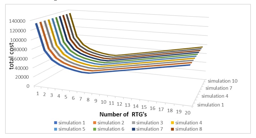
Therefore, in the case of 8 RTGs, the minimum cost can be achieved. So, in total, 4 QC are served for the unloading of the ships, a total of 32 RTGs is required and the total cost is 14975 * 4 + 24140 = 84040. To test the impact of the container storage configuration on the results, 10 simulation results are randomly selected to be compared with each other. The curves for the total cost function are shown below (Fig. 7). The number of RTGs, therefore, has a negligible effect on the cost of QC.
Fig. 7: Results of ten random simulations
Other numerical tests and analysis
In addition, numerical tests will be performed to examine the validity of the simulation performance. The purpose of these tests is to determine the relationship between certain main parameters and the number of RTGs. The cost calculation depends on: the unit cost of the vessel MC0 and the unit cost of the RTG VC0. There are several other parameters that affect the travel time in each cycle. The queue condition and the unloading volume of ship 1, can be simply represented by the total unloading of the number of containers divided by the number of CQs, as well as by the operating time of the unit of each type of crane.
Modification of the values of the unit cost of unloading the vessel and the unit cost of RTG.
The unit cost of QC and the unit cost of RTG vary depending on many factors, such as the port situation, the size and concessionaire of the terminals and the volume of operations, if there are rental contracts between the port authority and ship companies. However, depending on the actual situation, there must be a range within which these two cost values can fluctuate. MC0 can fluctuate between [5, 30], while VC0 can vary between [0.8, 3]. On the basis of these results, by combining these two values randomly, 10 tests are carried out and the results are presented in the following table:
Table 3: Optimal results with different unit costs (USD)
It can be seen that the optimal number of RTGs used in these simulations is around 8. Therefore, the best number of RTGs used is not sensitive to the change in cost in these ranges.
Modify the unloading volumes and the number of QC.
In this case, with the same operating time of the QC, the same speed of the RTG, the same size and the same definition of the two sites S1, S2, only the number of incoming containers and the number of QC served is changed. In general, the workload for the QC is between 200 to 600 containers for each ship, and each ship must be served by 2 to 6 QC. According to this practice, the tests with the different groups will be simulated several times to obtain the statistical results presented in the following table:
Table 4: Results of different numbers of containers and number of QC used
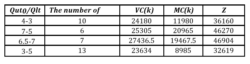
Modify the QC unit time report for unloading and loading
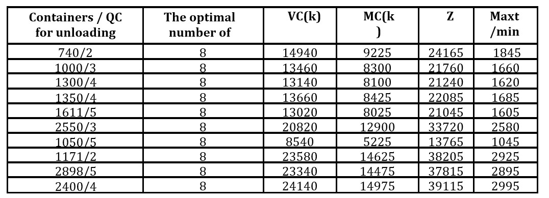
Keeping the same parameters from table 1 only the operation time for unloading and loading the QC is changed. The statistical results are presented in the following table:
Table 5: Results with different QC time unit
The optimal number of RTGs used in these simulations is deferent in each case. Therefore, the best number of RTGs used is sensitive to the change of the QC operation time.
Conclusion
According to the numerical tests carried out, the storage configuration of the containers has no effect on the best number of RTGs. Changing the unit cost (within a valid interval) or the number of QCs (within a valid range) has no effect on the best number of RTGs, and will only affect the total working time and costs. Changing the unit operating time of the QC for unloading (within a valid range) has a marginal impact on the best number of RTGs and it directly affects the results. The best number of RTGs also depends on the unit time of the QCs and the speed of the RTGs, which are the components of this equation [8]. In addition, even unit costs will not change the number of RTGs.
Agostino, I., Sousa, S., Frota, P., Daher, R., & Souza, A. M. (2019). Modeling and Simulation of Operations: A Case Study in a Port Terminal of Vale S/A. In New Global Perspectives on Industrial Engineering and Management (pp. 91-99). Springer, Cham. https://doi.org/10.1007/978-3-319-93488-4_11
Carboni, A., & Deflorio, F. (2020). Simulation of railroad terminal operations and traffic control strategies in critical scenarios. Transportation Research Procedia, 45, 325-332.
Chen, L., & Lu, Z. (2012). The storage location assignment problem for outbound containers in a maritime terminal. International Journal of Production Economics, 135(1), 73-80.
Guedj, C., Claret, N., Arnal, V., Aimadeddine, M., & Barnes, J. P. (2007). Evidence for 3-D/2-D transition in advanced interconnects. IEEE Transactions on Device and Materials Reliability, 7(1), 64-68.
Lee, D. H., Cao, J. X., Shi, Q., & Chen, J. H. (2009). A heuristic algorithm for yard truck scheduling and storage allocation problems. Transportation Research Part E: Logistics and Transportation Review, 45(5), 810-820.
Preston, P., Kozan, E., 2001. An approach to determine storage locations of containers at seaport terminals. Computers & Operations Research 28, 983–995.
Sauri, S., & Martin, E. (2011). Space allocating strategies for improving import yard performance at marine terminals. Transportation Research Part E: Logistics and Transportation Review, 47(6), 1038-1057.
Soriguera F, Espinet D, Robuste F (2006) A simulation model for straddle carrier operational assessment in a marine container terminal. JMaritime Res 3(2):19–34