The Financial Driver of Business Cycle Synchronization

Introduction

This paper contributes to the International Business Cycles literature by analyzing the effect of financial integration, trade integration and similarity of economic structures on business cycle synchronization (BCS). In particular, this paper addresses the question of whether financial integration has become the main driver of business cycle synchronization, as the empirical evidence presents mixed results regarding the relationship between financial integration and output comovement. This issue has important policy implications, specifically regarding the fulfillment of an optimum currency area (OCA), whereby the benefits of a currency union depend on the degree of synchrony of its members’ business cycles, as high similarity in economic fluctuations should minimize the effect of giving up national monetary policy and its ability for dampening idiosyncratic shocks (Darvas and Szapáry, 2008; Schiavo, 2008). In theory, similarity between business cycles would minimize the negative impact of the loss of national monetary instruments and the impact of exogenous monetary shocks induced by the monetary union authorities.

The concept of economic globalization is strongly linked to the pervasive economic and financial relationships observed worldwide since the 1990’s. Empirical evidence suggests that economic integration amplifies the transmission of global shocks and the international spillover of country shocks, leading to synchronizing effects across national business cycles. Indeed, numerous studies document a process of increasing comovement of business cycles between economies during the last decades (Antonakakis and Scharler, 2012; Belke, Domnick and Gros, 2017) as well as an increase in the influence of global factors over national business cycles (Kose et al., 2008; Kose et al., 2003), which have led some to argue for the existence of a global business cycle (Crucini, Kose and Otrok, 2011).What is driving the increase in the synchronization of business cycles around the world?. Many candidates have been proposed since the early 2000’s (Baxter and Kouparitsas, 2005).These are essentially related to the increasing integration of major international transmission channels such as trade (Calderon, Chong and Stein, 2007; Kollmann, 2019) and finance (Claessens, Kose and Terrones, 2012), as well as to the increasing similarity of economic structures (Pentecôte, Poutineau and Rondeau, 2013) and economic policies (Antonakakis and Tondl, 2014).

In the aftermath of the 2007-08 global financial crisis, a great body of research focused on examining the ability of financial markets to globally propagate shocks to the real side of economies. Standard theoretical literature of international business cycles suggests that Foreign Direct Investment (FDI) and the access to international financial markets can trigger a reduced level of comovement between countries as they stimulate specialization of production through the reallocation of capital according to countries’ comparative advantages. By allowing cross-border ownership of means of production and assets, financial integration provides investors with better insurance against production risk derived from higher exposure to asymmetric shocks (Schiavo 2008; Baele et al. 2004). Moreover, a positive productivity shock in one country is likely to attract investments from other economies and to increase sectorial specialization as long as the marginal productivity of capital and labor is increasing (Backus et al. 1995). Financial integration may affect the degree of business cycle synchronization by generating large demand, as well as, supply side effects. For example, saving and investment decisions could affect asset prices and business cycles in other countries via financial flows (Artis, Fidrmuc and Scharler, 2008). In this way, the supply of foreign capital can cause a positive correlation between source and target countries (Fidrmuc, Ikeda and Iwatsubo, 2012), amplifying the probability of an idiosyncratic shock to spillover towards other countries.

As for the negative side, corporate finance theories imply that negative productivity shocks should lead to capital withdrawals, amplifying output differences among financial integrated economies. A shock to bank capital in one country can force banks to reduce their lending to other countries, causing interconnected economies to experience an increase in the comovement of output (Kalemli-Ozcan, Papaioannou and Peydró, 2013). Furthermore, financial integration can facilitate the transfer of resources across countries through FDI by shifting capital from economies with negative shocks to economies with positive shocks. FDI enables countries to specialize (Kalemli-Ozcan, Sørensen and Yosha, 2003) so that a high degree of financial integration may actually reduce BCS.

It is not surprising to find that empirical evidence presents mixed results, taking into consideration the variety of variables and methods employed in order to measure financial integration. Following what is predicted by standard theories, a negative correlation between financial integration and output comovement is reported by studies like García-Herrero and Ruiz (2008), Claessens, Kose and Terrones (2012) and Antonakakis and Tondl (2014). However, several studies suggest a positive effect of financial integration on output comovement (Artis, Fidrmuc and Scharler, 2008; Inklaar, Jong-A-Pin and de Haan, 2008; Imbs, 2010). Additionally, a vast body of empirical research reported a historically high level of international comovement of real and financial variables following the 2007-08 global financial crisis (Banerji and Dua, 2010; Antonakakis and Scharler, 2012; Perri and Quadrini, 2018).

The discrepancies displayed by empirical studies may result from methodological disparities, whether due to differences in the adoption of proxy measures for financial and economic variables or in modeling their relationship. For example, cross-section studies which cover turbulent and calm periods, as (Imbs (2006), Kose, Prasad and Terrones (2003) and Otto, Voss and Willard (2001), find a positive correlation between financial openness and GDP comovement. Some studies suggest this positive relationship manifests strongly between economies sharing high levels of integration such as OECD economies (Otto, Voss and Willard, 2001; Imbs, 2010) and European economies (Schiavo, 2008; Antonakakis and Tondl, 2011). However, cross-section studies may suffer from not being able to account for country-specific factors and global shocks occurring over time, as argued by Kalemli-Ozcan, Papaioannou and Peydró (2013).

This paper foresees two major contributions. First, the level of financial integration in the BCS context is analyzed considering three dimensions simultaneously: (1) Price measure, represented by the interest rate term spread differential between each pair of economies, (2) Flow measure, represented by the foreign direct investment (FDI) intensity between each pair of economies and (3) Volume measure, represented by the financial openness of both economies in that “pair”. With this enlarged perspective, the aim is to capture extra dimensions of the financial integration between eventually relevant economies in the BCS context. Second, this approach differs from previous studies by adopting a structural equation model that allows gathering the main representative variables for each factor (financial integration, trade integration and similarity of economic structure), capture its common variance and then estimate its simultaneous direct and indirect effects on BCS. In principle, this approach should be able to provide a multidimensional view of the impact of the financial factor on BCS. The rest of the paper is structured as follows; it presents the methodological approach in section 2 along with data, variables and model specifications, it examines the empirical results and discusses its implications in section 3 and provides some concluding remarks in section 4.

Methodological Approach: The Structural Equation Model

In this paper, a structural equation model (SEM) is employed in order to estimate the effects induced by main BCS factors, which are modeled as latent constructs. A SEM consists of a structural model which relates the latent variables (factors) and factor models which set the relationship between latent variables and their observable indicators. This class of models suits this research particularly well, as BCS factors are not directly observable and therefore could hardly be measured by one single indicator. SEM enables the use of several proxy indicators for BCS factors, providing a mechanism of explicitly, taking into account the likelihood of measurement error in the observed variables. In addition, SEM also allows the simultaneous estimation of both direct and indirect effects of variables involved in the model.

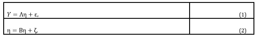
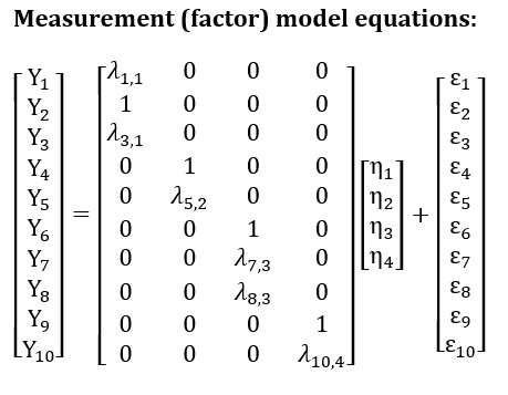
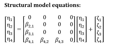
The SEM model proposed in this paper is represented by the following pair of equations (1) and (2), for each country-pair ( ) period-specific ( ) observation (for simplicity of notation, the subject subindex ( )) is suppressed:

where Y denotes the vector of observed variables,  is the vector of latent factors, is the matrix of factor loadings and  is the vector of pertinent residuals.  denotes the vector of latent disturbance terms and  represents the matrix of parameter coefficients linking latent variables, where is is assumed to be invertible. Residuals are assumed to be uncorrelated among themselves (  versus ) and with factors (  and  versus ), while factors are allowed to be contemporaneously interrelated, meaning that B is a not a diagonal matrix. Factors, observed variables and residuals are assumed to be normally distributed, which is a common standard in multiple regression models.

The observed variables covariance matrix  implied by (1) and (2) has the following form (Bollen, 1998):

denotes the vector of all model parameters, which includes all variances and covariances between independent variables as well as regression coefficients and factor loadings. The fit function of the model is estimated by the maximum likelihood method, by minimizing across the parameter space:

where S is the covariance matrix for observed items and  corresponds to the number of observed variables (number of elements of matrix Y in Equation 1). There is a growing literature applying factor models to the study of international business cycles. These studies typically focus on measuring the importance of broad factors of national business cycles and distinguishing between global, regional and country-specific components (Kose, Otrok and Whiteman, 2008; Aruoba et al., 2011; Bordo and Helbling, 2011). In this paper, factor models are made use of in order to (i) reassess the explanatory power of established BCS factors in the literature such as trading and financial channels and structural similarities, and (ii) examine if the financial channel has become the main driver of output synchronization.

Data, Variables and Model Specification

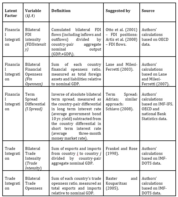
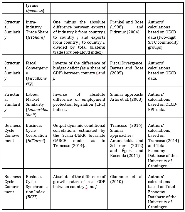
The mainly used variables are collected in the literature and fed to the explanatory latent factors; financial integration, trade integration and structural similarity. Table 1 provides detailed information on the variables employed by the model, its links to BCS literature and data sources.

In order to accommodate a complex view of financial globalization, the financial integration factor is allowed to be expressed as the common variance from three financial variables; bilateral FDI intensity (FDI Intensity), bilateral financial openness (Fin Openness) and the term spread differential (i Spread). The trade integration factor is measured by a bilateral flow measure (trade intensity) and a bilateral measure of the country-pair’s global exposure to trade (trade openness). The structural similarity factor accounts for sectoral similarity (proxied by intra-industry trade share), labour market similarity and similarity in economic policies (proxied by a measure of fiscal convergence).

Table 1: Variables description and data sources

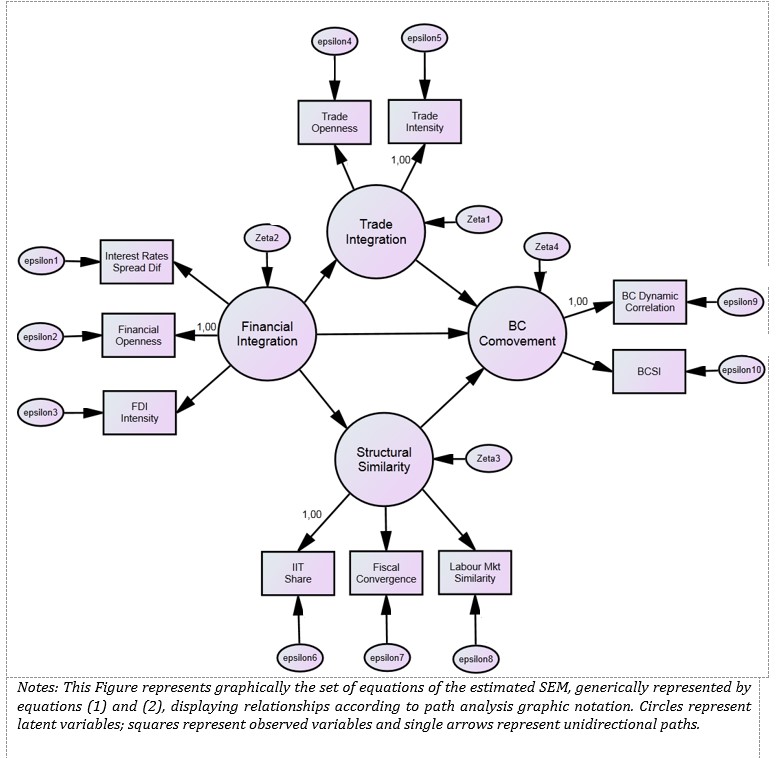
This paper examines if financial integration has become the common factor driving output synchronization in recent years. The specification chosen for SEM allows testing this viewpoint specifically, as financial integration becomes the only factor permitted to have an impact on other latent factors. Figure 1 presents a path diagram that provides a visual depiction of SEM specification. It discloses all relationships specified by the model in accordance to equations (1) and (2). Following BCS literature, this paper studies the effect of (i) financial and trade integration factors, acting as channels for the transmission of shocks, and (ii) structural economic similarities on the BCS.

The metric of the latent scale needs to be set for each latent variable in order to achieve model identification, as there is no “natural” metric underlying any of the latent variables. We define the metric for each BCS factor by setting to one the path going out to the representative variable adopted more often in BCS literature: Financial openness (Financial Integration factor), Trade intensity (Trade Integration factor) and Intra-industry trade share (Structural Similarity factor). With respect to Business Cycle Comovement factor, the representative variable is the Business Cycle Dynamic Correlation. It should be noted that, in order to detect possible bias resulting from this procedure, results from alternate specifications, generated by interchanging the variable used as scale for each factor, were examined. In the end, the scaling variables were kept as previously mentioned, as factors’ estimates have shown less sensitivity to scaling up on other variables.

Figure 1: Model Path Diagram

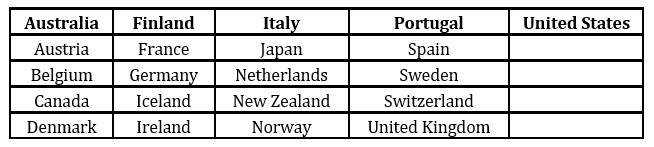
The number of variables (10) used in the model as well as data availability constraints conditioned the dataset in respect to the delimitation of the sample period and the set of countries. For example, the whole sample had to be limited to data up to 2011 so as to make use of the unique dataset of foreign assets and liabilities provided by Lane and Milesi-Ferretti (2007), in which latest data points are from 2011. SEM model in this paper uses annual data (3322 observations) for the period 1995-2011 from 21 advanced economies listed in Table 2.

Table 2: List of countries used in SEM Model

Empirical Results           

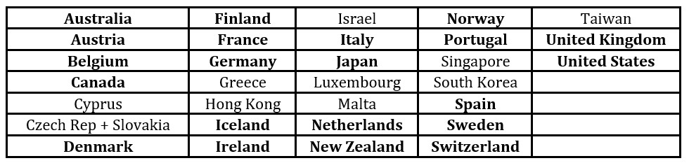
The study begins by examining the existence of a relevant common factor by running a principal component analysis (PCA) over the real output variance. This enables adding more countries to the dataset (see Table 3) and using a more representative sample of World GDP.

Table 3: List of Countries Used in PCA Analysis

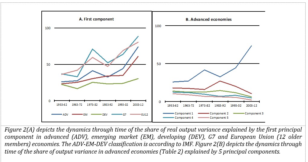
There is evidence that a major common factor has been increasingly influent over the past six decades, especially in advanced economies (see Figure 2A). Moreover, evidence plotted in Figure 2(B) suggests that the increase of the relative importance of the first component, observed from the 1990’s onwards, has occurred at the expense of the remaining four main considered drivers.

Figure 2: Principal Component Analysis of real output variance

Results suggest that a common factor has been driving output synchronization since the 1990’s. This paper proceeds to examine whether financial integration has become such a common factor. The specification chosen for the SEM allows testing this viewpoint specifically, as financial integration becomes the only factor permitted to have an impact on other latent factors.

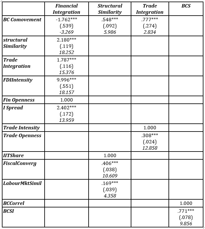
Tables 4-6 present the estimation results for the SEM derived from setting the interrelationships between variables in accordance to equations (1) and (2), as graphically represented in Figure 1. Table 4 and 5 breakdown the corresponding direct and indirect effects while Table 6 discloses estimates of total effects (direct and indirect effects).

Table 4: Model Estimates of Direct Effects

Notes: Standard errors and corresponding t-statistics are reported below the estimates.

Estimates of direct effects are all statistically significant at 1% level and show that bilateral financial integration, manifested as the common variance reflected by the three financial indicators, exhibits a negative and significant direct effect on BCS. This result may be indicative of reallocation of capital in a manner consistent with countries’ comparative advantages and also reflects the necessity to insure against national business cycles risk, in line with standard financial and economic theories and with various empirical results (García-Herrero and Ruiz, 2008; Kalemli-Ozcan, Papaioannou and Peydró, 2013).

This model allows financial integration to impact BCS through international trade and structural similarity. This is supported by the theoretical argument; that more financially integrated countries induce increased similarity of productive structures and intensification of trade relations (Backus, Kehoe and Kydland, 1995; Antonakakis and Tondl, 2014). Results displayed in Table 5 not only confirm these findings by identifying a positive relationship between financial integration and the remaining factors (structural similarity and trade integration), but also detect a strong positive indirect effect that exceeds the negative direct effect on BCS.

A breakdown of direct and indirect effects of financial integration on BCS, displaying patterns of possible conflicting signals, has been detected by other empirical studies (García-Herrero and Ruiz, 2008; Antonakakis and Tondl, 2014). However, the novelty from the results of this model refers to the positive net effect of financial integration on BCS. This divergence may stem from these studies being focused on FDI linkages, accounting for a subset of financial activity with a relatively smaller impact on real economy than the entire set of cross-border financial activities, which are represented by three indicators in this model; bilateral FDI intensity, bilateral financial openness and the term spread differential. The FDI intensity measure includes two-way FDI flows and is therefore able to capture bilateral interactions.

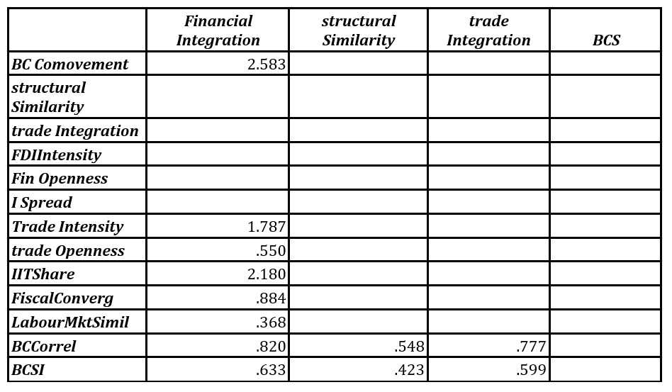
Table 5: Model Estimates of Indirect Effects

Notes: Following SEM methodology, indirect effects are computed as the product of the parameters of direct effects reported in Panel B. For example, the indirect effect of Financial Integration on BCS equals 2.583=1.787×0.777+2.18*0.548. 

On the other hand, variables represented by financial openness and the term spread differential provide bilateral outlooks about the global exposure to international financial markets faced by each country-pair. Results support the view that these variables display complementary but somehow different facets of the financial integration process, as shown by their different factor loadings estimates. Moreover, results are also consistent with the viewpoint (Adam et al., 2002; Baele et al., 2004) that price measures (term spread differential) and flow measures (FDI intensity) tend to be much more sensitive to changes in financial integration than measures based on volume positions (financial openness).

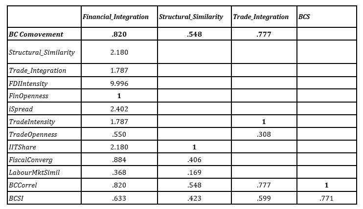
Table 6: Model Estimates of Total (Net) Effects

Notes: For each of the latent factors, there is one representative variable to which is attributed a coefficient equal to 1 (see above). Total Effects = Direct Effects (Table 4) + Indirect Effects (Table 5).

Results corroborate the positive and significant effect of trade integration on BCS that has been reported elsewhere (Artis, Fidrmuc and Scharler, 2008; Schiavo, 2008). Regarding bilateral trade relations, existent flows seem to matter more than just sharing a high degree of openness, as revealed by the difference in factor loading estimates. A similar picture is revealed by the effect of structural similarity on BCS. Although a higher degree of heterogeneity is revealed by factor loadings and error terms estimates, estimates from the structural similarity factor are positive and highly significant with respect to the structural model (effect on BCS) and to its measurement model (factor loadings), which is in line with existing literature (Duval et al., 2016).

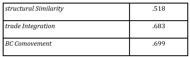
Next this paper examines how effectively BCS factors predict business cycle comovement in this model. Table 7 shows the squared multiple correlation (SMC) between each endogenous variable and the variables (other than residual variables) that directly affect it according to Figure 1. SMC correlations are analogous to R² indices corresponding to regression models for each equation, when all model equations are simultaneously estimated. SMC estimates suggest that financial integration factor variance explains a major part of trade integration (68%) and structural similarity (52%) variances. Moreover, BCS driving factors are jointly responsible for 70% of BCS variance according to SMC estimates. Consequently,  a strong and pervasive real effect of financial integration is found, which may suggest that Financil Integration factor plays a key role in the common factor disclosed by the PCA analysis detailed above (Figure 2).

Table 7: SMC

Notes: The table displays the squared multiple correlation of each dependent variable, disclosing the share of variance that is explained by the explanatory variables assumed by the structural equation model (see Equation 2).

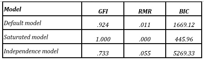
This model is tested by inspecting its adequacy through the observation of approximate goodness-of-fit indices. The majority of the fit indices devised by SEM literature are based on the known fact that in large samples, the minimization of Equation 4 approaches a chi-square distribution, if the model is correct and fitted to the covariance matrix (Kline, 2011). Three fit indices are computed; (1) the Goodness-of-Fit Index (GFI), which is an absolute fit index that estimates the proportion of covariances in the sample data matrix explained by the model, (2) the Root Mean Residual Square (RMR), which provides a measure of the mean absolute covariance residual; (3) the Bayes Information Criterion (BIC) to complement the analysis. Results from the approximate goodness-of-fit indices are presented in Table 8 and compared to two extreme baseline models. Following what is standard procedure in SEM literature, the results of the goodness-of-fit indices are displayed from the model (default model) alongside with results from the independence model, in which the observed variables are assumed to be uncorrelated with each other, and from the saturated model; one that perfectly fits the data as no constraints are placed on the population moments.

Table 8: Model fit indices

Notes: Values for Goodness-of-Fit Index (GFI), Root Mean Residual Square (RMR) and Bayesian Information Criterion (BIC).

While GFI is a goodness-of-fit index, RMR and BIC reflect the extent to which the model does not fit the data. As with many other descriptive indices, there is no strict norm for interpreting GFI values, nonetheless the result is consistent with the conventional view that GFI in the 0,90’s represents a good approximation of the data. On the other hand, RMR and BIC values are unexpectedly closer to the saturated model, as this model contains ten variables and it is known that BIC assigns a higher penalty to model complexity (Raftery, 1993).

Conclusion

This paper adds to the growing literature on the determinants of BCS by proposing a factorial multivariate approach to measure the financial integration impact on BCS. It is noted that financial integration has become a major driver of business cycle synchronization by promoting trade integration and economic similarity between countries.

Overall, the results favor some reconciliation between theory and empirical evidence. Allowing bilateral financial integration to load both on quantity measures (FDI intensity and financial openness) and price measures (term spread differential), a negative and significant direct effect on bilateral BCS is documented, in line with what would be expected by standard theories. However, major positive indirect effects of financial integration are found on bilateral BCS running through trade integration and structural similarity factors. Although such positive indirect effects have also been found elsewhere, the results in this paper point that their magnitude overrides the negative direct effect.

Policy makers may find these results providing valuable information in respect to the dynamics of economic integration, as a high degree of business cycle correlation is traditionally seen by the OCA literature as an important criterion to be met before joining a monetary union. As explained previously, similarity between business cycles could minimize the negative impact from the loss of national monetary instruments and the impact from exogenous monetary shocks induced by the monetary union authorities. Results lend some support to the endogenous hypothesis raised in literature that countries may be better candidates to join a monetary union ex post than ex ante (Schiavo, 2008). As the net positive effects from the financial and trade integration boost output convergence between monetary union members, these union members fulfill the standard criteria more effectively for an optimum currency area after joining the monetary union. The results are consistent with such viewpoint, which may facilitate the implementation of the common monetary policy in the monetary union, therefore generating a virtuous cycle.

Acknowledgment

The author Sofia Gomes gratefully acknowledges the financial support of Research Group of ISAG (NIDISAG).

References

• Adam, K. et al. (2002) ‘Analyse, Compare, and Apply Alternative Indicators and Monitoring Methodologies to Measure the Evolution of Capital Market Integration in the European Union’, Report to the European Comission.
• Adrian, T., Estrella, A. and Shin, H. S. (2010) ‘Monetary Cycles, Financial Cycles and the Business Cycle’, FRB of New York Staff Report, (421).
• Antonakakis, N. and Scharler, J. (2012) ‘The synchronization of GDP growth in the G7 during US recessions’, Applied Economics Letters, 19(1), pp. 7–11.
• Antonakakis, N. and Tondl, G. (2014) ‘Does integration and economic policy coordination promote business cycle synchronization in the EU?’, Empirica. Springer US, 41(3), pp. 541–575.
• Artis, Fidrmuc, J. and Scharler, J. (2008) ‘The transmission of business cycles’, Economics of Transition, 16(3), pp. 559–582.
• Aruoba, S. B. et al. (2011) ‘Globalization, the Business Cycle, and Macroeconomic Monitoring’, NBER International Seminar on Macroeconomics, 7(1), pp. 245–286.
• Backus, D., Kehoe, P. J. and Kydland, F. (1995) ‘International Business Cycles: Theory vs. Evidence’, Frontiers of Business Cycle Research, pp. 331–356.
• Baele, L. et al. (2004) ‘Measuring financial integration in the euro area’, Oxford Review of Economic Policy, 20(4), pp. 509–530.
• Banerji, A. and Dua, P. (2010) ‘Synchronisation of Recessions in Major Developed and Emerging Economies’, Margin: The Journal of Applied Economic Research, 4(2), pp. 197–223.
• Baxter, M. and Kouparitsas, M. A. (2005) ‘Determinants of business cycle comovement: a robust analysis’, Journal of Monetary Economics, 52(1), pp. 113–157.
• Belke, A., Domnick, C. and Gros, D. (2017) ‘Business Cycle Synchronization in the EMU: Core vs. Periphery’, Open Economies Review. Springer US, 28(5), pp. 863–892.
• Bollen, K. A. (1998) Structural equation models. John Wiley & Sons, Ltd.
• Bordo, M. D. and Helbling, T. F. (2011) ‘International Business Cycle Synchronization In Historical Perspective’, The Manchester School, 79(2), pp. 208–238.
• Calderon, C., Chong, A. and Stein, E. (2007) ‘Trade intensity and business cycle synchronization: Are developing countries any different?’, Journal of International Economics, 71(1), pp. 2–21.
• Claessens, S., Kose, M. A. and Terrones, M. E. (2012) ‘How do business and financial cycles interact?’, Journal of International Economics, 87(1), pp. 178–190.
• Crucini, M. J., Kose, M. A. and Otrok, C. (2011) ‘What are the driving forces of international business cycles?’, Review of Economic Dynamics, 14(1), pp. 156–175.
• Darvas, Z. and Rose, A. K. (2005) ‘Fiscal divergence and business cycle synchronization: irresponsibility is idiosyncratic’, Kozgazdasagi Szemle (Economic Review), 52(12), pp. 937–959.
• Darvas, Z. and Szapáry, G. (2008) ‘Business cycle synchronization in the enlarged EU’, Open Economies Review, 19(1), pp. 1–19.
• Duval, R. et al. (2016) ‘Value-added trade and business cycle synchronization’, Journal of International Economics. North-Holland, 99, pp. 251–262.
• Égert, B. and Kocenda, E. (2011) ‘Time-varying synchronization of European stock markets’, Empirical Economics, 40(2), pp. 393–407.
• Fidrmuc, J. (2004) ‘The Endogeneity of the Optimum Currency Area Criteria, Intra‐industry Trade, and EMU Enlargement’, Contemporary Economic Policy, 22(1), pp. 1–12.
• Fidrmuc, J., Ikeda, T. and Iwatsubo, K. (2012) ‘International transmission of business cycles: Evidence from dynamic correlations’, Economics Letters, 114(3), pp. 252–255.
• Frankel, J. A. and Rose, A. K. (1998) ‘The Endogeneity of the Optimum Currency Area Criteria.’, Economic Journal, 108(449), pp. 1009–25.
• García-Herrero, A. and Ruiz, J. M. (2008) ‘Do trade and financial linkages foster business cycle synchronization in a small economy?’, Moneda y crédito, (226), pp. 187–238.
• Giannone, D., Lenza, M. and Reichlin, L. (2010) ‘Business cycles in the euro area’, NBER Working Papers, (w14529), pp. 141–167.
• Imbs, J. (2006) ‘The real effects of financial integration’, Journal of International Economics, 68(2), pp. 296–324.
• Imbs, J. (2010) ‘The first global recession in decades’, IMF economic review, 58(2), pp. 327–354.
• Inklaar, R., Jong-A-Pin, R. and de Haan, J. (2008) ‘Trade and business cycle synchronization in OECD countries—A re-examination’, European Economic Review, 52(4), pp. 646–666.
• Kalemli-Ozcan, S., Papaioannou, E. and Peydró, J.-L. (2013) ‘Financial Regulation, Financial Globalization, and the Synchronization of Economic Activity: Financial Integration and Synchronization’, Journal of Finance, 68(3), pp. 1179–1228.
• Kalemli-Ozcan, S., Sørensen, B. E. and Yosha, O. (2003) ‘Risk sharing and industrial specialization: Regional and international evidence’, The American Economic Review, 93(3), pp. 903–918.
• Kline, R. B. (2011) Principles and practice of structural equation modeling. Guilford press.
• Kollmann, R. (2019) ‘Explaining International Business Cycle Synchronization: Recursive Preferences and the Terms of Trade Channel’, Open Economies Review. Springer US, 30(1), pp. 65–85.
• Kose, M. A., Otrok, C. and Whiteman, C. H. (2008) ‘Understanding the evolution of world business cycles’, Journal of International Economics, 75(1), pp. 110–130.
• Kose, M. A., Prasad, E. S. and Terrones, M. E. (2003) ‘How does globalization affect the synchronization of business cycles?’, The American Economic Review, 93(2), pp. 57–62.
• Lane, P. R. and Milesi-Ferretti, G. M. (2003) ‘International financial integration’, IMF Staff Papers, pp. 82–113.
• Lane, P. R. and Milesi-Ferretti, G. M. (2007) ‘The external wealth of nations mark II: Revised and extended estimates of foreign assets and liabilities, 1970–2004’, Journal of International Economics. North-Holland, 73(2), pp. 223–250.
• Otto, G., Voss, G. and Willard, L. (2001) ‘Understanding OECD output correlations’, RBA Research Discussion Papers. Sydney: Economic Research Department, Reserve Bank of Australia, (2001–05), pp. 2001–05.
• Pentecôte, J.-S., Poutineau, J.-C. and Rondeau, F. (2013) Trade Integration and Business Cycle Synchronization in the EMU: the Negative Effect of New Trade Flows. Center for Research in Economics and Management (CREM), University of Rennes 1, University of Caen and CNRS.
• Perri, F. and Quadrini, V. (2018) ‘International Recessions’, American Economic Review, 108(4–5), pp. 935–984.
• Raftery, A. E. (1993) ‘Bayesian model selection in structural equation models’, Sage Focus Editions, 154, p. 163.
• Schiavo, S. (2008) ‘Financial integration, GDP correlation and the endogeneity of optimum currency areas’, Economica, 75(297), pp. 168–189.
• Trancoso, T. (2014) ‘Emerging markets in the global economic network: Real(ly) decoupling?’, Physica A: Statistical Mechanics and its Applications, 395, pp. 499–510.

Appendix

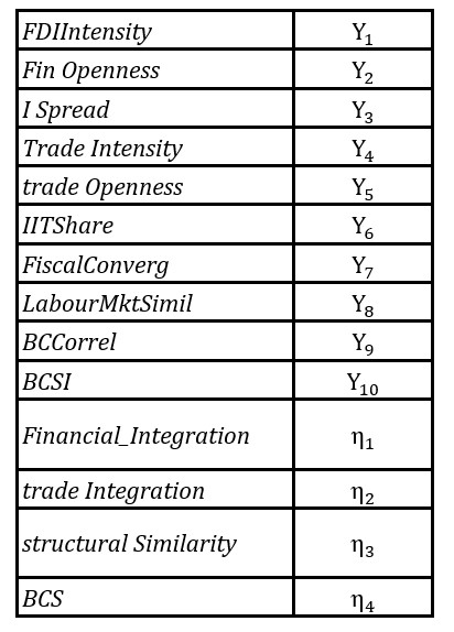
In this section we present the relationships assumed in our structural equation model, as formalized in equations (1) and (2) and depicted in the path diagram exhibited in Figure 1. As explained in section 2, the model is defined by two submodels – the factor/measurement model (Equation 1) and the regression/structural model (Equation 2). We refer to the equations of the model using the following notation for observed (Y)and latent (η)variables: