Approximation of Experimental Data for Inverter Output Power and Research on the Distribution of the Load between Different Inverters of String Topology for Photovoltaic Power Plants
Power Electronics Department, Technical University-Sofia, Kliment Ohridski Blvd., Bulgaria
Volume (2013),
Article ID 336432,
International Journal of Renewable Energy & Biofuels,
16 pages,
DOI: 10.5171/2013.336432
Received date: 22 April 2013; Accepted date: 26 May 2013; Published date: 19 October 2013
Academic Editor: Awang Bin Jusoh
Cite this Article as:
Mihail Antchev and Angelina Tomova (2013), "Approximation of Experimental Data for Inverter Output Power and Research on the Distribution of the Load between Different Inverters of String Topology for Photovoltaic Power Plants," International Journal of Renewable Energy & Biofuels, Vol. 2013 (2013), Article ID 336432, DOI: 10.5171/2013.336432
In this paper, the authors have done a processing of experimental data for the generated output power of two photovoltaic parks by means of different methods. An approximation of the data is done for the output power during a good day (with maximum solar radiation) by a Sum of Sinusoidal Functions, and during a bad day (small solar radiation) – by a sum of Gaussian functions. The paper presents also a research on the distribution of the load between different inverters of a string topology on-grid photovoltaic system. It is done by means of MATLAB software computer approximation of experimental data from the monitoring of photovoltaic generators, in order to estimate and prolong the lifetime of the different inverters of the string topology of the system. Based on results of the research a schedule for exchange of the inverters is proposed, in order to optimize the lifetime of the entire system.
With regards to the policy for development and promotion of the generation of electricity from renewable energy sources, governments have deployed different strategies and regulations in order to encourage the investments in this area. This favorable regulatory frame results in many installations for energy generation from renewable energy sources, mainly from photovoltaic modules. The huge dissemination of those PV generators focuses the research interest on two main directions, both related to the optimization of the performance, and the reliability and efficiency of the installations.
Research in the field of the system performance is mainly related to definition and implementation of new or advanced methods for maximum power point tracking algorithms. In the research paper of Blanes, et al., (2013) is presented a practical implementation of the maximum power point tracking estimation algorithm and the PV curves. It is very suitable for monitoring and control use. The one of Shenoy, et al.,(2013) describes an optimization method for a power production of PV systems, resulting in improved system reliability, simplification of the MPPT process and protection, and monitoring capacity improvement. Nousiainen, et al.,(2013) investigated the properties of a PV generator as well as the effects of its behavior to the interfacing inverter.
Storey, et al., (2013) presented a research on the optimization of PV production which proves that major optimization would come from the environmental and installation factors. This is the reason that the work in the second direction-optimization of the reliability and the efficiency is focused on the analysis of different topologies. As Meneses, et al., (2013) mentioned in their comparative review of topologies for photovoltaic AC-module applications or by Gu, et al., (2013) and their very reliable and performing transformless topology of grid-connected PV inverter. In order to predict the failures of the systems, researches are done in the field of the calculation and prediction of these events. The paper of Harb and Balog (2013) proposes a methodology to calculate the mean time before failure of a photovoltaic inverter taking into account the environmental changes, Estefany De Leon-Aldaco, et al., (2013) analyzed PV on-grid converters, calculated their failure rates and proposed four different prototypes, based on the prediction of the behavior. Reliability prediction is very important for the operation and maintenance of the grid-connected PV generators especially for estimation of inverters lifetime and the possibility of its prolongation by good distribution of the load to the inverters and their exchange between different strings from these with smaller load to those with bigger load and vice-versa. Such an estimation method of the lifetime of an on-grid inverter and prediction of a failure prior to its occurrence is researched in the study of Huang and Mawby (2013). As main parameter of each system, the investigation on the efficiency of the inverters in very important and different methods for its measurements can be used as presented in the paper of Aarniovuori, et al., (2013). Efficiency of the grid-connected PV systems could vary according to the weather conditions as it is mentioned by Alajmi, et al., (2013) who proposed an improvement method in this case. In the research study by MacAlpine, et al., (2013) it is presented a software analysis of the operation of PV systems under nonuniform conditions, results of which are focused on some suggestions for the efficiency and performance improvement.
Prediction method of the output power and the efficiency of a solar system is proposed by Yan and Chan (2012). It introduces a Gaussian shape prediction of a typical day generation of a solar system. Another prediction methods presented by Perpinan, et al., (2007) are based on mathematical equations of the models of the PV array and the inverter using time-domain and irradiance domain integrals. The Herrmann, et al., (2006) rely on the statistic methods to predict the output power of a photovoltaic system. Other methods are observation and analysis of the output data of a PV system for a long period, on the basis of which an analytical model is developped as mentioned by Marcos, et al., (2011).
The majority of the recent researches use Gaussian approximation of the results of the daily power measurements independantly of the atmospheric conditions. There was no research on another approximation methods, which can provide better accuracy of the approximation. There is also no comparision of the approximation results in case of different solar irradiation for instance. Guassian approximation is applicable for approximation of measured data under specific atmospheric conditions and under others it might be feasible to use more accurate approximations.
It is well-known that the output power of a photovoltaic system depends on different conditions such as solar radiation, humidity, pressure, wind speed, etc. For the purpose of the below presented research two cases have been chosen – a very good day, when the output power injected into the grid is close to the maximum, and a very bad one when only a small part of the installed inverter power is used. The research methodology is the following: records of the measurements of the monitoring system of the photovoltaic systems are used. On this basis is done a comparative analysis of two approximation methods for the good and the bad day and is defined the most appropriate one. After that it is possible to do further more accurate forecasts on the output energy of the entire system as well as on its inverters’ load.
This paper is focused on two directions. First the definition of the best approximation method of the output power of a grid-connected PV system by means of MATLAB software in case of different weather conditions, expressed by the solar irradiation value and fluctuation, so that the analysis and the prediction of the behavior of the system could be easy and reliable. Second major topic is the analysis of the distribution of the load between different inverters of one system by approximation of their output power in order to predict their lifetime and to develop exchange schedule of those inverters within the system in order to prolong the lifetime of the entire system.
The rest of the paper is organized as follows. The description of the analyzed systems and experimental results for the total output power, used for the definition of the most suitable approximation methods are presented in Section II. In Section III is presented the choice of the characteristics’ approximation methods. Section IV describes the analysis of the distribution of the load between the different inverters, and Section V concludes the presented results.
Description of the Systems
For the purpose of the research, two photovoltaic systems have been monitored- PV1 and PV2. Both systems have similar installed power so that the comparison of their parameters would be realistic- 84kWp and 95kWp. They are connected to the low voltage utility grid- 0.4kV and are both composed of 5 strings connected to 5 inverters according to the string topology presented in Fig.1. The 95kW system- PV1 is composed of four inverters each of them of 20kW and one inverter of 15kW. To each inverter are connected four strings of 21 panels with unit power of 235Wp polycrystalline technology. The 84kW system- PV2 is composed of two inverters of 20kW and three inverters of 15kW. The 15kW inverters are fed with three strings of 16 panels of 195Wp, and the 20kW inverters are fed with three strings of 18 panels of 195Wp each of them.
Fig.1: String Topology on-grid Connection
Experimental results for the total output power, used for the definition of the most suitable approximation method
In Fig.2 below are presented the results from the monitoring of those two systems. Monitoring data is composed of power charts for two days with different solar irradiation. The first one 17th March 2013 when the solar irradiation was high and relatively stable, called for the purpose of the analysis “good” day, and the second one 18th March 2013 when the solar irradiation is low and very fluctuating called “bad” day. In the charts for both systems and days are presented the output power of the system, the average power of the system, the solar irradiation and the PV panels’ temperature.
Fig.2: Power Charts-Hour Chart for 17.03.2013 And 18.03.2013 A) and B)-for PV1, C) and D) – for PV2
“Copyright of Solarity BG Ltd. 2013, Used by Permission”
Choice of Characteristics’ Approximation Method
In this part is presented an approximation of the two photovoltaic systems for a day with relatively stable solar irradiation-17.03.2013- the “good” day. For both systems are applied two approximations- one with Gaussian function and one with function composed of sum of sinusoidal functions. In Fig.3 are shown the results as follows: on the upper diagrams- the original curve of the output power, Gaussian approximation and Sum of Sin Functions approximation, on the bottom diagram- the residuals for each of the two approximations which show the quality of the approximation method. For each system approximation are obtain approximation functions- denoted by, , ,where the numbers in the indexes (1 or 2) show the system number and the letters (g or s) show the approximation method- Gaussian or Sum of Sine Functions.
Fig.3: Approximation of the Output Power of Two Photovoltaic Systems for the “Good” Day by Two Methods- Gaussian and Sum of Sinusoidal Functions: A) PV1 System; B) PV2 System
The methodology of the approximation is the following: monitoring data for both days for both PV systems is extracted in a suitable numeric form and then uploaded to MATLAB by a small command file. As a result of the execution of the approximation program file, preliminary define by the authors, we obtain the approximation functions and coefficients of each term of the expression. This methodology is used for all the approximations presented in this paper.
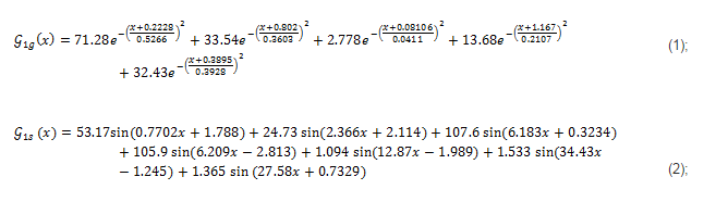
The approximation functions for Gaussian approximation and Sum of Sin Functions approximation for the first system- PV1 are presented in (1) and (2):
The approximation functions for Gaussian approximation and Sum of Sin Functions approximation for the second system- PV2 are presented in (3) and (4).
Based on the results presented above, it is obvious that for the output power of both systems for the conditions of stable solar irradiation the Sum of Sin Functions approximation is better than the Gaussian approximation. The residuals are smaller and closer to zero, and residual picks are smaller and less present.
The quality of the approximation can be expressed by the RMSE (Root-Mean-Square Error) for both approximations for both PV systems. For PV1 RMSE of the Gauss approximation is 2.152, and the RMSE for the Sum of Sin Functions approximation is 1.3. For PV2 RMSE of the Gauss approximation is 2.17, and the RMSE for the Sum of Sin Functions approximation is 1.9. It is obvious that in both cases Sum of Sin Functions approximation presents better fitting results less important residuals which is in line with the here above statement in the previous paragraph.
The same approximations- Gaussian and Sum of Sin Functions, are next done for the same two PV systems, but for a day with smaller solar irradiation with huge fluctuations-18.03.2013- the “bad” day. In Fig.4 are shown the results as for Fig.3: on the upper diagrams- the original curve of the output power, Gaussian approximation and Sum of Sin Functions approximation, on the bottom diagram- the residuals for each of the two approximations which show the quality of the approximation method. For each system approximation are obtain approximation functions- denoted by , , , where the numbers in the indexes (1 or 2) show the system number and the letters (g or s) show the approximation method- Gaussian or Sum of Sine Functions.
Fig.4: Approximation of the Output Power of Two Photovoltaic Systems for the “Bad” Day by Two Methods- Gaussian and Sum of Sin Functions: A) PV1 System; B) PV2 System
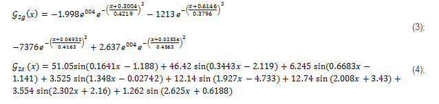
The approximation functions for Gaussian approximation and Sum of Sin Functions approximation for PV1 are presented in (5) and (6) and for PV2 in (7) and (8):
Based on the approximation results, we can conclude that in case of small and variable solar irradiation the output power function is better approximated by Gaussian approximation than by Sum of Sin Functions approximation. This is also clear by the residuals graphs where the residuals of the Gaussian fit are much closer to zero and present lower picks.
As a measure for the quality of the fit in case of cloudy day, we use the same error factor RMSE. For PV1 RMSE of the Gauss approximation is 1.805 and the RMSE for the Sum of Sine Functions approximation is 1.886. For PV2 RMSE of the Gauss approximation is 1.89 and the RMSE for the Sum of Sine Functions approximation is 3.366. In this case, we can conclude that Gaussian approximation is more suitable even though the difference in the RMSE between the two approximations for PV1 is less pronounced.
Analysis of the Distribution of the Load between the Different Inverters
The next part of the research is focused on each separate inverter composing the photovoltaic system. For this purpose the PV1 is used.
Fig.5: Comparison Charts-Hour Chart For PV1 for: A) 17.03.2013- “Good” Day; B) 18.03.2013-“Bad” Day
“Copyright of Solarity BG Ltd. 2013, Used by Permission”
The power of the entire system is 95kW. It is distributed into four inverters each of them of 20kW and one inverter of 15kW. To each inverter are connected four strings of 21 panels with unity power of 235Wp polycrystalline technology. The further analysis considers the four inverters of same power- 20kW even though approximations are done for all the 5 inverters. The data used for the analysis and presented in Fig.5 is also for the two days- “good” and “bad” and is obtained from the monitoring system of PV1.
The analysis for each of those four inverters present two major ideas: approximation of the power curve for the “good”and the “bad” day and evaluation of the produced energy by each of them for each of those two days. The choice of the approximation methods regarding the solar irradiation is based on the conclusions done in the previous part i.e. the “good”day with Sum of Sin Functions fit and the “bad” day- Gaussian fit.
Analysis for Inverter 1
Fig.6: Results for Inverter 1 for the “Good” Day: A) Approximation; B) Energy Evaluation
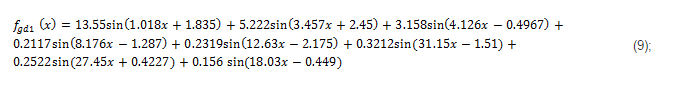
In this part is presented the analysis for the first inverter. In Fig.6 a) is shown the approximation result for the “good” day to which is related the function described in (9) and in Fig.6 b) is presented the curve of the produced energy for this same “good” day according to the approximation function and to the data from the monitoring.
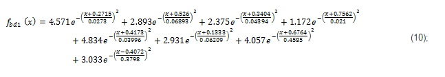
Fig.7 a) presents the approximation result for the “bad” day to which is related the function of the Gaussian fit described in (10) and in Fig.7 b) are shown the curves of the produced energy for this same “bad” day according to the approximation function and to the data from the monitoring.
Fig.7: Results for Inverter 1 for the “Bad” Day: A) Approximation; B) Energy Evaluation
Analysis for Inverter 2
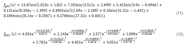
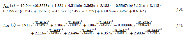
The presentation of the research on the Inverter 2 is done the same way as for the previous inverter-in Fig.8a)- the Sum of Sin Functions approximation for the “good” day – described by (11); in Fig.8b)- the energy graphs before and after the approximation; in Fig9.a)- the Gaussian fit for the “bad” day- , presented in (12); and in Fig9.b)- the energy produced by the inverter according to the approximation data and the monitoring data.
Analysis for Inverter 3
This part shows the results of the analysis for the third inverter. In Fig.10 a) is presented the approximation result for the“good” day by Sum of Sin Functions – described in (13) and in Fig.10 b) is presented the curve of the produced energy for this same “good” day according to the approximation function and to the data from the monitoring. In Fig.11 a) is presented the approximation result for the “bad” day to which is related the function of the Gaussian fit described in (14) and in Fig.11 b) are shown the curves of the produced energy for this same “bad” day according to the approximation function and to the data from the monitoring.
Analysis for Inverter 4
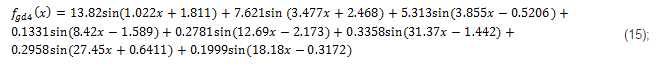
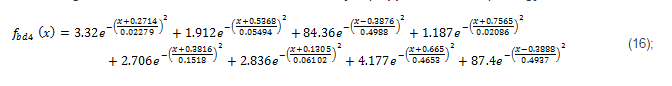
Analysis results for the fourth inverter are presented in Fig.12 and Fig.13 as follows. In Fig.12.a)- the Sum of Sin Functions approximation for the “good” day – described by (15); in Fig.12.b)- the energy graphs before and after the approximation; in Fig13.a)- the Gaussian fit for the “bad” day- , presented in (16); and in Fig13.b)- the energy produced by the inverter according to the approximation data and the monitoring data.
Analysis for Inverter 5
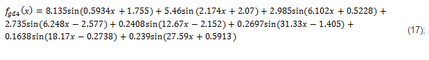
The presentation of the research on Inverter 5 is done the same way as for the others- in Fig.14a)- the Sum of Sin Functions approximation for the “good” day- described by (17); in Fig.14b)- the energy graphs before and after the approximation; in Fig15.a)- the Gaussian fit for the “bad” day- , presented in (18); and in Fig.15.b)- the energy produced by the inverter according to the approximation data and the monitoring data.
Fig.14: Results for Inverter 5 for the “Good” Day: A) Approximation; B) Energy Evaluation
Fig.15: Results for Inverter 5 for the “Bad” Day: A) Approximation; B) Energy Evaluation
In order to summarize the results concerning the produced energy by each inverter for the set of the two days- good andbad, the results on hourly basis are presented in Table 1. From them one can notice that Inverter 1, Inverter 2, and Inverter 4 have similar energy production during the “good” day. Meanwhile the production of the third inverter is lower than those for the three others with approximately 10%. During the “bad” day all four inverters have similar production of energy.
Table 1: Energy Produced by Each of the Five Inverters for the “Good” and the “Bad” Day
The output power of each string of a photovoltaic system depends on different conditions- solar radiation, humidity, pressure, wind speed, etc. During the two days of the experimental research the conditions of the operation of the different strings have been approximatevely similar- absolutely sunny day (good day) and absolutely cloudy day (bad day).
Regarding to this information we can conclude that Inverter 3 is less loaded that the other 3 inverters of same power rate-Inverter 1, Inverter 2 and Inverter 4, in case of stable and high solar irradiation, which presents 90% of the days for the region where the PV1 system is situated. In that case his operational lifetime will be longer than those of the other three inverters and a good opportunity to prolong the operational lifetime of the entire PV system would be to periodically exchange the place of the inverters or connect the less loaded one- Inverter 3 at the place of the most loaded Inverter 2, and so on.
It is clear that the operational conditions of the strings during the days of the year are random and the conclusion which is made is valid under the condition that the major part of the days in the region where the system operates is whether good or bad. However, it is possible to forecast up to a certain level, the possibility of reliable operation of the entire system because of the uniform loading of its inverters. Conclusion
This paper presents research on on-grid power converters. The research is focused on two major directions- approximation of the output power of the inverters depending on the solar irradiation values and stability and comparison and analysis of similar inverters regarding their load based on the produced energy aiming to propose optimization of the operational lifetime and the performance of the system. Research results prove that the best approximation method for this first case of high and stable irradiation is the Sum of Sin Functions approximation, and in case of low and variable irradiation, it is the Gaussian approximation.
The analysis of the results is based on explicit measurements of the output power of each inverter by means of the monitoring of the system. It results in the authors’ conclusion that higher accuracy of the approximation during the “good” day is reached by Sum of Sine Functions approximation, and the well-known Gaussian approximation presents more accurate approximation results for the “bad” day. Based on this conclusion for the presented photovoltaic systems it is presented suitable the scheduling connection between some of the inverters.
The proposed method can be used for proceeding of the results of the monitoring systems of other photovoltaic systems by means of the proposed approximations, aiming to define the possibilities of more uniform loadability of the inverters. The proposed expressions and approximation methods can be used for forecast purpose by using forecast distribution of the days’ results for a longer period.
References