1Bucharest University of Economic Studies, Bucharest, Romania
2Informatics and Economic Cybernetics Department, Bucharest University of Economic Studies, Centre for Industrial and Services Economics, Romanian Academy, Bucharest, Romania
Volume 2023,
Article ID 557970,
Journal of Eastern Europe Research in Business and Economics,
12 pages,
DOI: 10.5171/2023.557970
Received date: 15 September 2022; Accepted date: 21 February 2023; Published date: 24 March 2023
Academic Editor: ILIE Constantin
Cite this Article as:
Delia BĂLĂCIAN and Stelian STANCU (2023)," An Economic Analysis of Neural - Based Techniques Applied for Energy Consumption Prediction", Journal of Eastern Europe Research in Business and Economics Vol. 2023 (2023), Article ID 557970,
DOI: 10.5171/2023.557970
Energy consumption is of tremendous importance in modern society because of its impact on both climate change mitigation and the economy. In order to develop methods for reducing energy loss and carbon emissions, research has focused on improving building energy monitoring and planning. To achieve climate neutrality by 2050, the European Commission has set ambitious targets for increased energy efficiency in buildings and the increased use of renewable energy sources. The stakes of having robust prescriptive mechanisms to support the usage of renewable energy have grown once again in the context of the recently announced action plan REPowerEU. The research analyzes a dataset with over 8,000 entries and 123 variables, 14 of which were collected from an individual building and the rest were derived from the dataset by calculating the minimum, maximum, mean, standard deviation, hour, day, month, and wind direction. The case study compares the best models from two architectures of Artificial Neural Networks, Feed Forward and Long Short-Term Memory, in terms of performance by calculating the values for R-Squared, Mean Absolute Error and training time. In addition, comparisons between Adam and Adagrad as weight correction optimization functions are made. The key findings of the study indicate that the two types of architectures have similar performance metrics but Feed Forward Neural Network models are preferred to the Long Short – Term Memory ones given that the training time is significantly shorter while the R-Squared value is similar. The analysis continues with looking at the learning curves for each optimization function, unraveling that Adagrad is a better option for both types of neural networks than Adam.
Keywords: Energy Consumption, Artificial Neural Networks
Introduction
Energy consumption has become a widely discussed subject in the modern society due to its undeniable impact on the global climate change mitigation initiative as well as its important role in the proper functioning of the economy. As a result, many changes have been implemented in the building energy management system, with the goal of reducing both energy loss in the network and the emissions of greenhouse gases. In order to achieve this, prediction models are essential and play an important role in the decision-making process of the stakeholders, as well as in the planning and monitoring of these systems. The European Union has long been paying attention to the issues associated with building energy consumption and those regarding the climate objectives set for 2030: the member states have sought to improve the energy efficiency of buildings both by retrofitting old structures and by constructing new buildings according to more energy efficient designs. Moreover, the introduction of green energy sources has also become a viable and increasingly popular solution in the effort to reduce energy consumption and combat climate change.
In 2022, the European Commission put forth REPowerEU, a strategic strategy to quicken current energy policies. The strategy was developed at a time when the conflict between Russia and Ukraine had already begun and had dramatically altered European geopolitics and significantly influenced the economies of European nations and the European Union. The EU’s dependence on Russian natural gas and oil is detrimental, and the energy market is one of the economic sectors that is greatly affected. Russia’s economic and strategic influence through its resources is manifested in the negotiation of its state based on what it can provide, the energy dependence of European countries, thus countermeasures are mitigated in the absence of alternatives (European Commission, 2022). The inherent instability of renewable energy sources, which are promoted for long-term usage, is the main source of fluctuation in the energy production process. To support the decision-making process and the management of the energy system as a whole, the predictive tools employed in the energy industry must become more accurate and faster.
This study offers a comparison of two Artificial Neural Networks (ANNs) in terms of performance, accuracy, and efficiency. These ANNs are known as Feed-Forward Neural Networks (FFNN) and Long-Short Term Memory (LSTM). Because these methods can process vast amounts of data to provide direction for future actions, there is significant potential for their use in applications relating to energy usage. The availability of data and the ability to access computing power have contributed to the rise in popularity of machine learning techniques, which are the foundation of artificial neural networks (ANNs).
The case study presented here is intended to support research in the energy sector and its greater objective of minimizing the costs associated with energy supply interruptions, while also improving the way predictions are made in the energy field. This is an important step in the process of sustainably and efficiently responding to society’s energy needs, particularly in the case of renewable sources. The challenges faced in energy production management can be daunting, but with the right strategies and understanding, the chances of meeting society’s energy demands can be increased. By understanding and improving the way predictions are made in the energy field, the chances of sustainably and efficiently responding to society’s energy needs are higher than ever before.
Literature Review
The discipline of artificial intelligence is mostly comprised of machine learning techniques, which opened the way for the development of today’s advanced models, known as ANNs. Machine learning algorithms investigate input-output correlations using or without mathematical models. By feeding input data to well-trained machine learning models, decision makers can achieve satisfactory prediction output values (Lai, et al., 2020). The phase of data preprocessing is extremely important to the process of machine learning and has the potential to considerably improve its overall effectiveness (Provost & Fawcett, 2013). First, the technology of machine learning employs three unique learning techniques: supervised learning, unsupervised learning, and reinforcement learning. In the training phase of supervised learning, labeled data are utilized. Unsupervised learning refers to the method of autonomously categorizing unlabeled data based on predetermined criteria. Consequently, the number of clusters is often defined by the clustering criterion employed. Reinforcement learning gives a formulation of the problem in which an agent interacts with its surroundings across a series of time steps. At each time step, the agent receives feedback from the environment and must choose an action to send back to the environment through a mechanism (Zhang, et al., 2021).
Recent years have seen a flourishing of deep learning techniques, which is represented by ANNs. This has evolved as a result of the advancement of technology in both hardware and software. These methods are able to bring about characteristic nonlinear features as well as high-level invariant data structures. As a consequence of this, it has found applications in a wide variety of fields, where it has proven to be successful (Gu, et al., 2018). Due to their computing capabilities, ANNs have been widely used for making predictions in the energy area, as well as because the interest in developing better predictive tools in energy system management has been growing rapidly (Sina, et al., 2022). Gating is a mechanism that helps the neural network decide when to forget the current input and when to keep it for subsequent time steps. In today’s modern society, one of the gating mechanisms that is utilized the most frequently is Long-Short Term Memory neural network, which is a recurrent model. A recurrent neural network is a form of neural network that is capable of learning relationships between two distant points in a sequence. This sort of network is known as a deep neural network. Data can be classified, clustered, and predicted with the help of these advanced algorithms (Fukuoka, et al., 2018).
Among the most critical issues that the energy productions from renewable sources will face in the near future is energy supply. The integration of renewable energy sources into present or future energy supply architecture is referred to as renewable energy supply. Renewable energy systems will be able to tackle critical parts of today’s energy concerns, such as boosting energy supply reliability and managing regional energy shortages. However, due to the significant volatility and intermittent nature of renewable energy, managing several energy sources demands the pursuit of increased prediction accuracy and speed (Lai, et al., 2020). Managing the fluctuation of renewable energy statistics is thus an ongoing challenge. High-precision energy monitoring helps improve the efficiency of the energy system. Energy forecasting technology is critical in national economics and the development of energy system strategies (Solyali, 2021).
The adoption of alternative energy sources as a strategy for mitigating the negative effects of climate change and global warming is gaining favor. In an effort to improve the predictability of renewable energy sources, a number of different methods of prediction have been developed (Lai, et al., 2020).
The review paper discusses the procedures utilized in machine learning models for renewable energy forecasts, such as data pre-processing methods, parameter selection methodologies, and prediction performance evaluations. The mean absolute percentage error and the coefficient of determination were used to evaluate renewable energy sources.
During the last ten years, there has been a surge in interest in machine learning, data mining, and artificial intelligence (Shetty, et al., 2020). Researchers are able to investigate the energy consumption of buildings using the neural-based modeling approach, which does not require them to have prior knowledge of the industry. As a result, the researchers are able to develop models that ultimately meet the need outlined by industry professionals. The frameworks that have been described at the European level are providing support for neural and other data analytics-based solutions. On a worldwide scale, this type of frameworks is driving digital transformation through legislation and financing. Therefore, energy research is in an advantageous position to progress and expand making use of the most cutting-edge methodologies, artificial neural networks.
Methodology
An artificial neural network is a mathematical model of a system made up of nodes and connections between them, similar to how the brain is made up of neurons and synapses. The purpose of the artificial neuron is to take the input data, adjust it based on the associated weights, and then aggregate the outcomes for each input data . The activation function is then applied to the sum at the input layer of the artificial neuron, and the result is passed to the next layer. Consequently, it is essential to recognize that the activation function governs how input is turned into output at each layer of an artificial neural network. Mathematically, the activation function of a neuron is a nonlinear function that turns the neuron’s inputs into a distribution. Every ANN has an input layer and an output layer, but the number of hidden layers can vary based on how complex the network is. Aside from that, each ANN has a set of parameters that must be set in order to get a result. The weights of the neurons, the activation functions, the number of epochs, etc. are all part of the parameters. These are decided during the learning or training phase of the network. There are several ways to do this, which can be put into two main groups: supervised learning and unsupervised learning. Briefly, techniques in the first group use a data set whose output is known, and the algorithm learns how to classify new data or calculate numerical values that show the relationship between the variables being studied by using the regression method. Techniques from the unsupervised learning category are used to analyze and sort data without knowing in advance what kind of data they are. Clustering, association, and reducing the number of dimensions, are all part of this category (Delua, 2021).
Feed-Forward Neural Networks (FFNN)
FFNN is the fundamental kind of deep artificial neural network architecture, which was inspired by the way the brain functions. This strategy enables you to send information and process the intricate flow of information from one neuron to the next. The neural network concept we know today evolved from a famous machine learning technique known as the perceptron (Rosenblatt, 1960), which in turn developed through Warren McCulloch and Walter Pitts’ research.
The perceptron is a part of the neural network that takes values named X as input and uses a function to decide what to do with them. Rosenblatt suggested that the output data should be made based on the weights (w) that were given to the input data. These weights show how important each value is in the decision model. Lastly, after the model’s importance weights are applied to the input data, the perceptron is related to a set threshold, defined as a parameter, to generate an output.
In his book, (Nielsen, 2019) defined the manner in which the output is generated, using a function for the perceptron. In other words, the perceptron is a component that makes decisions according to the weights assigned to decision criteria. In the developed model, the input data associated with a decision criterion is given greater consideration the greater the weight. Additionally, the decision threshold for obtaining an outcome influences the model’s precision. Thus, by modifying the weights and threshold of the perceptron function, various parameter combinations and, consequently, decision models are created.
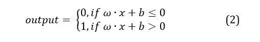
Equation. 1. Relation of determining the output at neuron-level, where is the associated weight and is the input data Another variant of defining the perceptron is by discussing about the bias of the perceptron, i.e., the negative value of the decision threshold of the outcome. From this point of view, bias can be thought of as a way to measure how quickly the perceptron can reach the value of 1.
Equation. 2. Relation of determining the output at neuron-level by introducing bias, where is the associated weight, is the input data and is the bias of the perceptron The multilayer perceptron neural network (MLP) is a common example of an FFNN created by integrating multiple perceptron layers. By default, MLP consists of three layers in which information flows from the input layer to the hidden layer to the output layer. Deep neural networks consist of neural networks that contain numerous hidden layers.
Contrary to the early emergence of the artificial neural network concept, this technology did not begin to prove its potential until four decades later. The concept of backpropagation (Rumelhart, et al., 1986) triggered growing interest in ANN, which essentially meant that the weights of each neuron were adjusted according to the actual outcome compared to the predicted result. The retrieved information is extremely valuable since the synaptic weights determine the significance of the input to the ANN. In other words, information travels from the output layer to the input layer when backpropagation is used. The output of a neural network depends on the flow of data through a collection of interconnected components. Each of these elements is designed such that a little increase in its output value influences the increase (or decrease) of the output values of all subsequent units up to the output of the network.
Long-Short Term Memory (LSTM)
LSTM is a type of ANN developed by integrating a memory cell into the hidden layer to manage the time series memory information. It has the ability to process time series data, but it minimizes the information transformation and the gradient problems (Hochreiter & Schmidhuber, 1997). The architecture for this type of ANN supports long-term dependencies on learning by including input, output, and forget gates.
The LSTM memory cell’s state is determined by the combination of the outputs of two of these gates: the forget gate represents the amount of information from the previous instant that can be preserved, while the input gate governs the amount of information and stimulus that will be merged together in response to the current input. One of the primary functions of the output gate is to control the flow of information transmitted for cell status (Lawal, et al., 2021). The transmitted data is directed to different cells in the hidden layer using the control gates. This allows for the selective recall and removal of past and present information. The LSTM, in contrast to the FFNN, can remember things over the long term and does not have the gradient descent problem.
The tanh activation function computes the input data and returns a value between -1 and 1, whereas the sigmoid activation function, as described in the preceding section, conducts identical operations but returns a value between 0 and 1. At this stage, the forget gate determines which information from the prior cell state is retained, based on equation (4), in which xt represents the input vector to the network at the reference time step t, Uf is a matrix of the weights of the input gate, ht-1 stands for the previous hidden state input, Wf is a matrix of the weights of the forgetting gate cell for the prior hidden state and bf is the associated bias:
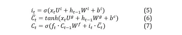
The input gate is formed by two mathematical layers: the first determines the new data which is to be stored in the cell’s state and this is described by equation (5). This layer functions similarly to the forget gate meaning that both the current state input and the previous state cell output are passed through a sigmoid function. The function takes into consideration the weights and bias for the present input and also for the output from the previous cell. The second layer functions in the same manner but applies the tanh activation function (equation 6) and the bias and weights are specific to this layer. Equations (6) and (7) describe how the information is processed for the new candidate values to be stored in the cell state and how finally the weights and bias from the previous cell state are taken into account in this computing process.
where Ui is the matrix of weights for the input gate, Wi is the matrix representing the weights of the input gate cell used for the prior hidden state and bi is the associated bias, is the new candidate for the cell state, Ct is the new cell state, ft represents the activation vector for the forget gate and it represents the activation vector of the input gate.
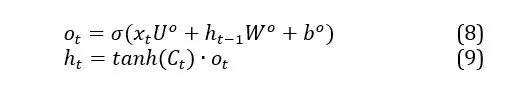
The next steps refer to the forget gate vector, which is multiplied by the prior state cell vector to determine the information from the previous cell state to be kept. Using the newly computed cell state Ct, the current input xt and the prior hidden state input ht-1, a new hidden state is then calculated. The newly determined cell state Ct is governed by a tanh activation function and is multiplied by the output vector to obtain the new current hidden state.
where ot is the output vector, Uo and Wo represent the matrix with the weights of the output gate and that associated with the prior hidden state, respectively, and finally ht is the current hidden state. For each of the new time steps taken into consideration, the present cell state Ct, also known as long-term memory, and the hidden state ht, generally known as short-term memory, are computed. The output of each time step is obtained through short-term memory (Foltean & Glovațch, 2021).
In a nutshell, the LSTM adjusts the values of the cell state and hidden state vectors given the input vector xt in addition to controlling the internal flow of information through the gates. These vectors will also be a part of the LSTM input set at time t+1, where t represents the current moment. Information flow control is employed to make the cell state act as a long-term memory, while the hidden state functions as a short-term memory. Actually, the short-term memory, the hidden state, and also recent past knowledge, the input vector, are used by the LSTM cell to update the long-term memory. Additionally, it uses the long-term memory to update the short-term memory. The hidden state discovered at t moment is also the output of the LSTM unit at that moment. In other words, it is what the LSTM offers to the outside world in order to complete a specific task. In other words, how well the LSTM performs depends on the behaviour.
Results and Discussion
The analysis and information presented in this paper was extended from the research done previously on this subject (Bălăcian & Stancu, 2022). Particularly, the results were discussed in more detail in this section and provide more insight into the performance analysis of the ANNs.
The dataset on which the neural network techniques were applied considers energy consumption data for a building, expressed in kWh or equivalent. Also, data related to the context existing at the time of recording the value for consumption are taken into account: air and morning temperature (degrees Celsius), degree of cloud cover (oktas), rainfall (millimeters), atmospheric pressure at sea level (millibars/hectopascals), direction (0 – 360 degrees) and speed (meters/second) of the wind. It should be mentioned that the values recorded for the target variable, energy consumption, and the descriptive variables, i.e., those containing data on the context of the consumption recording, are real. In addition to these, new descriptive variables were created, based on the existing ones, to capture more data for the neural network algorithm to use to extract information: the minimum, maximum, mean and standard deviation values for air temperature, wind speed, precipitations; also, the date on which the energy consumption value was recorded provided new variables for the type of day (weekday or weekend), month (January – December), hour (0 – 23), day of the week (Monday – Sunday) or day of the month (1 to 31). The added data values are relevant to the training process because more information is fed into the neural network. The increased volume of input data translates into improved predictions of the target variable – energy consumption. Therefore, the probability of obtaining accurate models from training ANN models rises.
In this study, the parameters used to compare the performance of the models are R – Squared, Mean Absolute Error (MAE) and the training time of the model. R-Squared indicates the confidence in the quality of the prediction, MAE determines the accuracy of it by calculating the difference between the predicted value and the actual one for each data entry in the models, and the training time refers to the speed of processing the data fed into the model. Each individual model is characterized by a number of epochs, a batch size and two hidden layers of neurons, each having a number of neurons.
The analysis is focused on the comparison between the functions for optimization of the weight correction. There is no need to adjust the adaptive optimizers. Adagrad applies a small adjustment to the learning rate for frequently occurring features and a large adjustment for the rare ones, allowing the network to capture information about uncommon traits while assigning them an appropriate weight. The rate at which each parameter is taught new information is adjusted in light of past gradients. Because the weights cannot be updated when the learning rate is too low, the possibility of a low learning rate across numerous steps due to accumulated gradients is relevant. By considering a fixed number of historical gradients, Adam reduces the probability that the network’s learning rate would drop so low that it stops improving.
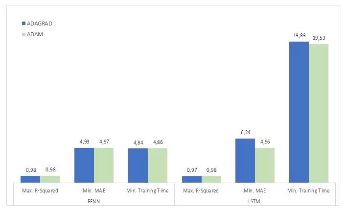
Due to its less complex architecture and input data processing, the FFNN has a far quicker training period than the LSMT model. The amount of time it takes to produce an output is significantly affected by the presence of input, output, and forget gates. Consequently, the FFNN model appears to be more appropriate for producing predictions fast and with an acceptable level of accuracy in the example of the selected building for the energy consumption dataset. Change in performance for each ANN model type is shown to be determined by the optimization functions, as it can be obseved in Figure 1.
Fig 1. The maximum value for R-Squared, the minimum value for MAE and the shortest training time for each optimization function, grouped by the ANN model type
Source: Author’s own research
When using Adam as the optimization function, the LSTM architecture achieves results that are comparable to those of FFNN. Even so, when Adagrad is used as the optimization function, the FFNN achieves the lowest Mean Absolute Error value (4,93) from all the models. The R-Squared differences between the two models are negligible and will not be used as a deciding factor. Both FFNN and LSTM benefit more from the Adam optimization function because, in an actual business context, it is more important to minimize prediction errors. In addition, training time is a crucial performance metric because of the need of producing precise results in situations when fast data processing is computationally demanding.
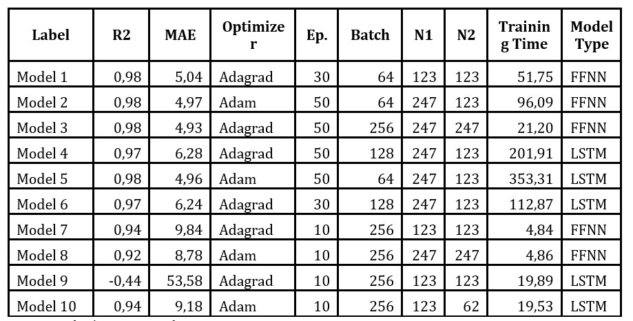
In Table 1 are presented the results obtained for each model in terms of the performance metrics. There are 10 models instead of 12 because some models meet the criteria for multiple performance metrics. More precisely, models 2 and 5 have the maximum value for R – Squared and the minimum for MAE from all the other computed models but, in the table, they are presented only once, having identical characteristics.
Table 1. Description of the models which have the best performance in terms of maximum R – Squared, minimum MAE or minimum training time from Figure 1, where R2 = R-Squared value, Optimizer = the optimization function applied, Ep= number of epochs, Batch = the number of neurons in a batch, N1 and N2 = the hidden layers
Source: Author’s own research
All the selected models have statistically acceptable values for R-Squared, between 0,92 and 0,98, except for model 9 (-0,44). The negative value for R-Squared means that the model could not reach a reliable results for this combination of parameters, where the optimization function was Adagrad, the epochs were set to 10, the batches of neurons at 256 neurons and the two layers of the neural networks at 123 neurons each. The current situation, in which a large amount of data to energy management systems are available, requires neural – based models that can give valuable results in a short amount of time, and FFNN is better suited to this particular objective.
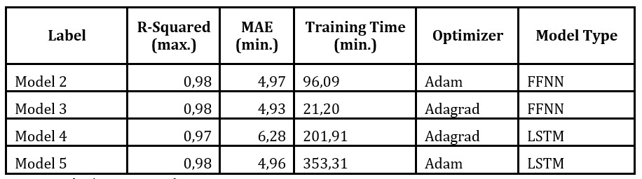
By selecting the highest values for R – Squared for each type of ANN and for each optimization function, four models stand out that are presented separately in Table 2. This performance measure does not fluctuate significantly. Further, the business need influences the choice of the best approach in terms of training performance and the prediction quality. For the latter, the values for MAE are similar generally and only for Model 4 the value is significantly greater. By contrast, the values for the training time vary greatly and separate the two architectures greatly. Overall, this more detailed analysis supports the idea that FFNN, used with Adagrad as a function for optimization of the weight correction, is a more economically responsible option.
Table 2. Description of the best two models for each architecture in terms of performance
Source: Author’s own research
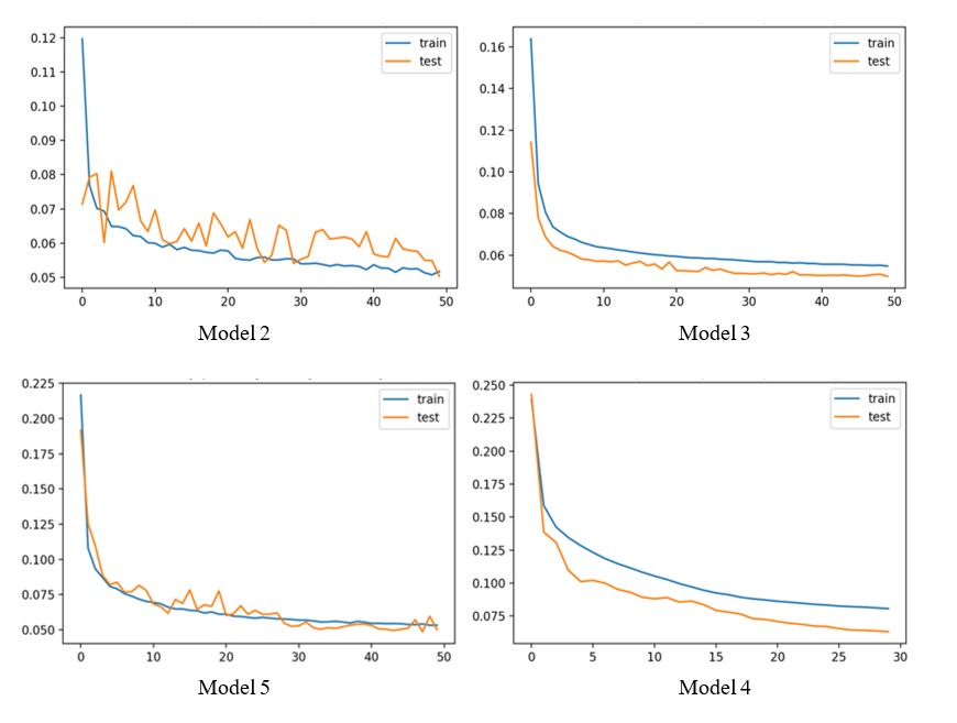
Then, the learning curves for the best models for each optimization function from Table 2 are shown in Figure 2. In the left side of the figure, it can be observed how the adaptive optimizer Adam varies for both FFNN and LSTM models as it considers a certain number of fixed gradients from the past and has a higher overall learning rate than Adagrad. This occurs because Adagrad affects the learning rate relatively little for often occurring features and significantly more for rarely occurring features. As can be seen in the representations on the right side of Figure 2, the learning rate is updated based on prior gradients and hence is smoother for both FFNN and LSTM models.
Fig 2. The learning curves of the best performing models for FFNN and LSTM architectures (first and second row, respectively) and for each optimization function, Adam in the left column and Adagrad in the right column, from Table 1
Source: Author’s own research
In the case of the four learning curves of the models compared in Figure 2, Adagrad performs better, even if the value for the R – Squared metric is slightly smaller when applied in a FFNN (0,97). Then, a comparison between the shapes of the learning curves of both optimizers reveals that Adagrad has fewer and lower spikes, that indicates this function for optimization of the weight correction is more reliable.
Conclusion
The use of renewable energy on a broader scale could be facilitated by incorporating predictive tools into building energy consumption planning and monitoring systems. The obstacles encountered in the pursuit of a more energy-efficient economy and optimal natural resource management are mostly associated with the unpredictability of renewable resources, the computing power required to process the available data, and the accuracy of the prediction models’ outputs. In order to reach the ambitious energy goals recently established by the European Commission, the predictability of energy consumption problems should improve.
The performance of the Feed Forward Neural Network and Long – Short Term Memory applied in this paper is comparable, as measured by R-Squared, allowing for a comparison of the two models. In addition, the Mean Absolute Error value and training time resulting for each model are provided in order to compare the precision and speed of each model type. In this instance, the performance of both neural network architectures is similar, but FFNN has a shorter training time and a lower MAE value.
Moreover, by looking at the learning curves of the best models for each ANN and each function for optimization of the weight correction, valuable insights were extracted: even if the value for R – Squared might be slightly lower and the ones for MAE and training time higher, the Adagrad function is more reliable, compared to Adam where strong variations are noticed for the case analyzed. As a result, the findings and analyses presented in this paper can help stakeholders in the energy industry find ways to differentiate themselves while reducing expenses and improving the quality of their systems and devices.
References
Bălăcian, D. and Stancu, S. (2022), ‘An Economic Approach On The Comparative Analysis Of FFNN And LSTM In Predicting Energy Consumption’, The Proceedings of the 40th International Business Information Management Association (IBIMA), ISBN: 979-8-9867719-0-8, 23-24 November 2022, Seville, Spain
Delua, J. (2021), ‘Supervised vs. Unsupervised Learning: What’s the Difference?’. [Online] NA [Accessed 4 September 2022] Available at: https://www.ibm.com/cloud/blog/supervised-vs-unsupervised-learning
European Commission (2022). ‘REPowerEU: A plan to rapidly reduce dependence on Russian fossil fuels and fast forward the green transition’. [Online] European Commission [Accessed 3 September 2022]. Available at: https://ec.europa.eu/commission/presscorner/detail/en/IP_22_3131
European Commission (2022). ‘The Recovery and Resilience Facility is the key instrument at the heart of NextGenerationEU to help the EU emerge stronger and more resilient from the current crisis’. [Online] European Commission [Accessed 4 September 2022]. Available at: https://ec.europa.eu/info/business-economy-euro/recovery-coronavirus/recovery-and-resilience-facility_en
Foltean, F. S. and Glovațch, B. (2021), ‘Business Model Innovation for IoT Solutions: An Exploratory Study of Strategic Factors and Expected Outcomes’, Amfiteatrul Economic, 23(57), 392 – 411
Fukuoka, R. et al. (2018). ‘Wind Speed Prediction Model Using LSTM and 1D-CNN’, Journal of Signal Processing (22), 207-210
Gu, J., Wang, Z., Kuen, J., Ma, L., Shahroud, A., Shuai, B., Liu, T., Wang, X., Wang, G., Cai, J. and Chen, T. (2018). ‘Recent advances in convolutional neural networks’. Pattern Recognition, 77(C), 354–377
Hochreiter, S. and Schmidhuber, J. (1997). ‘Long Short-term Memory’. Neural computation 9(8):1735-80
Lai, J.-P., Chang, Y.-M., Chen, C.-H. and Pai, P.-F. (2020). ‘A Survey of Machine Learning Models in Renewable Energy Predictions’, Applied Sciences (100. 5975), 1-20
Lawal, A., Rehman, S., Alhems, L. M. and Alam, M. M. (2021) ‘Wind Speed Prediction Using Hybrid 1D CNN and BLSTM Network’, IEEE Access(9), 56672–156679
Nielsen, M. (2019). ‘Chapter 1. Using neural nets to recognize handwritten digits’. [Online] NA [Accessed August 2022]. Available at:
Provost, F. and Fawcett, T. (2013). ‘Data Science for Business: What You Need to Know About Data Mining and Data-Analytic Thinking’, O’Reilly Media, Inc., United States of America
Rosenblatt, F. (1960). ‘Perceptron Simulation Experiments’. Institute of Electrical and Electronics Engineers (IEEE), 301-309
Rumelhart, D., Hinton, G. and Williams, R. (1986). ‘Learning representations by back-propagating errors’. Nature (323), 533–536
Shetty, D., Harshavardhan, C.A., Jayanth, MV., Shrishail, N., and Mohammed, R.A. (2020), ‘Diving Deep into Deep Learning: History, Evolution, Types and Applications’, International Journal of Innovative Technology and Exploring Engineering (IJITEE), 9 (3), 2835-2846
Sina, A., Leila, A., Csaba, M., Bernat, T. and Amir, M. (2022), ‘Systematic Review of Deep Learning and Machine Learning for Building Energy’, Frontiers in Energy Research, (10), 1-19
Solyali, D. (2021), ‘A Comparative Analysis of Machine Learning Approaches for Short-/Long-Term Electricity Load Forecasting in Cyprus’, Sustainability, 12(9), 3612
Zhang, A. C., Lipton Z., Li, M. and Smola, A. J. (2021). ‘Dive into Deep Learning’, Online, arXiv:2106.11342.