Customer Demand Forecast Using Time Series Approach

Introduction

Nowadays managers need data all the time to analyze what happened in the past, what will happen in the future, and try to make strategies and take decisions in real time that will affect the future of the company, especially when we are living in an unpredictable time period.

In this context we can we use different tools to collect data and statistical instruments that can help us model the phenomena in such a way that will provide the management of the information needed.

In this paper we aim to present a statistical method that can help the company in getting future predictions based on the historical data. Making predictions for what might happen in the future, means for a company a potential commercial benefits (Wang R., et. al., 2021).

More specifically, according to the data access we could get, we will predict the sold volumes for the next years, using time series method. The historical data are coming from the realised sales budgets from a company in the glass mould manufacturing area.

The objective of the research is to use and explore a model that can help organisations to preditct future sales and make decisions that will affect the performance of the organisation so in this way, through this paper, we contribute to the sales forecasting and time series method literature.

The forecasting process is actually an urgent need in many industries such as finance, healthcare, weather and transportation, and time series method can reppresent one of the key methods to solve problems (Wang R., et. al., 2021). More specific, through sales forecasting for example, companies can plan further the marketing activities, the production planning, purchasing and so on, in this way they can reduce future losses (Fan Z. P., et. al., 2017).

When companies are making sales plans, they can also take into consideration the macroeconomic indicators such as national market and economic factors that can drive the sales forecast (Zhang C. et al., 2019) for the long-term (Gao J. et all., 2018). In order to use macroeconomic indicators, we must consider a strong correlations between the sales volumes (the dependent variable ) and the  macroeconomic indicators (Zhang C. et al., 2019).

The paper is structured as follows. In the first section we will present the litterature review where we will emphasize different concepts about forecasting, predictions time series and budgeting. In the second section we will present the data collected, the model and time series processes. The third section presents the results obtained. In section four, we present the conclusion, and, in the last section, the oportunities for future research.

Litterature Review

The forecasting process represents a financial projection of the future based on objective or subjective methods (Laval V., 2018). Forecasts are made based on the information on how the variables have behaved in the past and the assumption that the patterns from the past will continue also in the future (Hannagan T. J., 1991).

According to Jain L. D. C and Malehorn J. (2006), there are 3 main types of pattern models that we can use to forecast a phenomena:

– Cause-Effect model: here we are talking about the existence of a cause (called driver or independent variable) and an effect (called dependent variable); here practically we determine the relationship between the variables and project them into the future, the most used here are the regressions as statistical technique;

– Critical model: this model is used especially when we do not have previous data for analysis, using specific procedures to make a prediction. Here the most known models are: Analog (a similar variable can be used as a basis for forecasting), Delphi (is done with the help of an expert group);  also, the authors Sagaert Y.R. et. al. (2018) are highlithing that expert information can lead to improving the forecasting performance, Diffusion (the prediction is made based on the product life cycle), PERT (performance evaluation review technique, where the forecast is done with the help  of an expert in the field who will provide 3 estimates: pessimistic, optimistic, most likely) and the Survey (represents the primary data that come from questionaires);

– Time Series model: this model works on the basis of extrapolating data from the past and starts from the assumption that the same pattern will continue in the future.

The basis of a forecast is the data we have available; based on this, we can also select the correct model (Jain L. D. C and Malehorn J., 2006).

Through the analysis of the time series, we can find useful information hidden in historic records. A time series is the value of a certain type arranged in chronological order. Time series can also be defined as a set of random variables arranged in a chronological order represented as X1; X2; Xt (Wang R., et. al.,  2021) and the author  Gong X. (2016) is mentioning also that a time series is a sequence of data points that are typically measured at successive and uniform time frames.

Time series analysis and forecasting are very much used in business for tactical, strategic, or operational planning and management (Sarfo P. A., et. al., 2015).

The general form of a time series is (Anghelache C., Manole A., 2012):

Yi = f (ti),

Where,

Yi = values of the studied variable

ti = numeric values of the time variable

The first time the time series model was introduced was in 1927, by the statistician Yule, where the the Autoregressive (AR) method uses the previous variable data to predict the performance of the next period. It is also called autoregression, as it always used the same variable. This model can be applied to systems that have relatively large data correlations in the prediction sequence (Wang R., et. al.,  2021).

1. Walker, in 1931, proposed the Moving Average (MA) model and established the hybrid model based on the AR model as ARMA. ARMA represents the classic time series forecasting model. This model is acceptable for stationary (means there is no trend or seasonal effects) single-variable time series modeling (Gonçalves J. N.C. et. al., 2021).

ARIMA model (Autoregressive Integrated Moving Average Model) was firstly introduced by Box and Jenkins in 1960 to forecast a non-stationary time series (Thanh-Lam N. et. al., 2013) into stationary series through appropriate order calculations and then using the ARMA model, commonly known also as ARIMAX (Gonçalves J. N.C. et. al., 2021).

Time series usually can include four influencing factors or components (Balakrishnan N.R., et. al., 2017):

– Trend: represents the upward or downward movement of data over time, may be influenced by factors such as market competition, technological development, prices;

– Seasonal variations: can occur at certain intervals of time within a year and may be above or below average demand, for example the increased sales of certain products during the winter holidays;

– Cyclical variations: these are patterns that appear over several years as a result of changes due to recurring and disappearing factors, after which they return at a certain time interval. For example, most countries’ economies experience high growth cycles after a relatively short period of growth or even recession. The cyclical variation can be seen as a hidden component in the trend and often cannot be predicted separately (Wang R., et. al.,  2021);

– Random, irregular components: they are caused by unforeseen events such as: wars, fires, pandemics.

They do not follow any pattern, and, for this reason, we cannot really include this component to predict future values.

The assumption underlying the construction of the models is that the chronological series are determined by systematic and not random causes (Cărbunaru B., Băcescu C., 2013). In order to make predictions theese components have firstly to be isolated, this process of isolation is called time series decomposition or time series analysis (Caraiani C. et. Al., 2010). There are two general approaches of decomposing a time series into its components (Balakrishnan N.R., et. al., 2017):

– The multiplicative type model assumes that the value of the prediction is the product of the four components of the time series;

– The additive model gathers the time series components together to provide an estimate.

The model of the chronological series of multiplicative type is based on the relation (Caraiani C. et. al., 2010):

M = T x S x C x R

And the additive type model is based on the following:

M = T + S + C + R

where,

T represents the trend;

S represents the seasonal component;

C represents the cyclic component;

R representsthe random, irregular component.

Further in this study we will realise the forecast of the volumes that are forecasted to be produced and, using the time series model, we will analyse the data and we will explain each step followed as well as the results.

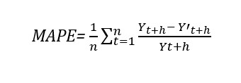
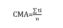
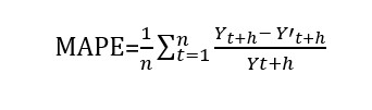
In the current  literature, in order to measure the accuracy  of the forecasting models, we often come across the calculation of the  Mean Absolute Percentage Error (MAPE), (Sagaert Y. R., et. al, 2017):

where,

Yt+h is the actual sales (the original data) and Y’t+h is the forecast values.

The authors Seval E. and Nursel O. (2017) shows a classification of the MAPEs indicators in order to determine the level of the prediction accuracy. A MAPE value that is less or equal to 10% represents the highest forecast accuracy. Between 10% and 20% there is a good accuracy, beetween 20% and 50% the accuracy is feasible and for a MAPE ≥50% the accuracy is low.

Ivert L. K. et. al., (2014) are also highlighting that, when measuring the planning accuracy, the metrics for the forecast error  should be at least 20% for the statistical forecast and 50% for the manual forecast.

Methodology and modeling setup

The current study aims to model and forecast the future demands, that means the volumes that are going to be produced and sold, from a company in the glass mould manufacturing area, using time series.

We want to mention that primary data are an important aspect of this research, as they will define the model we will work with. According to the data access that we managed to get we could obtain the information from the sales realised budgets and based on the the security policies of the company we will not mention its name. We can also mention that the company provides a complete range of mould parts for glass container production (for cosmetic ware, pharmaceuticals, table ware, jars, bottles for fruit juices, beers and spirits). The company offers the equipment for any shape in a wide variety cast irons or aluminum bronze, using various welding techniques.

Sales forecasting is very important in production, transportation and other activities, but also in the decision-making at all levels of the company. The importance of sales forecasting process has always been recognized by practitioners and academics (Sohrabpour V. et. al., 2021). The lack of forecasts or imprecise forecasting can lead to excess of inventory or loss of sales, which of course can force extra costs on the company (Lawrence M., et al., 2000).

So companies can reduce their losses in the production planning by increasing the sales forecasting (Marshall P., et al. 2013), and the results of the future predictions provide guidance to the managers (Seval E., Nursel O., 2017).

Most of the forecasting techniques use time series techniques that predict the behavior of future sales (or demands) assuming that the level, trend and seasonal fluctuations will follow the same rules in the future.

For the study, data have been collected from the actual sales budgets from the last 5 years representing the sold volumes of the company. The production portfolio of this entity has many items and the target product choosen for the research is the glass mould used for cosmetic ware, pharmaceuticals, table ware, jars, bottles for fruit juices, beers and spirits.

The data were collected via an enterprise resource planning (ERP) system, for each month and each year, so there is no month missing that should be replaced with proxy data. 

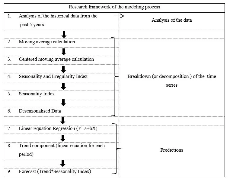
The research framework that was followed in order to predict the future sales of the company starts with the analysis of the historical data from the four past years, where we analysed the trend of the series, the existance of the seasonality variation, the cyclic component  and the random component. Then the moving average and the centered moving average was calculated followed by obtaining the seasonality and irregularity index. The seasonality index was then extracted in order to deseasonalize the data; the linear equation regression was calculated for the purpose of obtaining the trend component and the final forecast of the model.

Further, we illustrate the research framework for a better understanding and we will describe each step followed in the model.

Fig.1 : Research framework

(Source: author’s processing in Microsoft Word)

Analysis of the historical data for the past four years

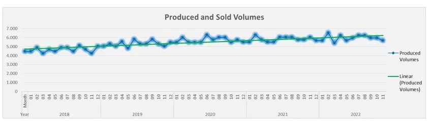
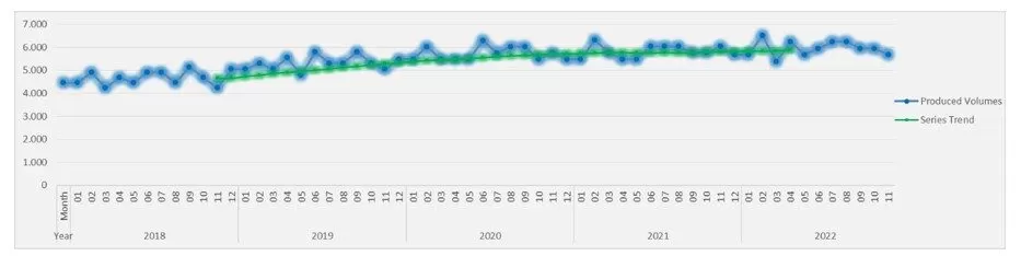
Analysing the historical data, represented also graphically in figure no.2, we can observe the trend, elements of seasonality, and no random components. On the horizontal axis, time is represented, and on the vertical axis, the variable Yf(t) represented the numerical values of the time variable.

We can see that the overall trend of the sold volume is increasing (in picture below represented by the green line). We can also highlight that every year, quarter 1 shows increases in the volumes, and quarter 2 decreases, this is the characteristic of the seasonality component (specific to each field of activity). In the year 2020, when the Pandemic started in Europe, we can observe a slight decrease in March, April, and May compared to the other years. No outlier can be noticed in the graphic; outliers means extreme and unusual values (Jain L. D. C and Malehorn J., 2006).

Fig. 2 : Historical data and their trend

(Source: author’s processing in Microsoft Excel)

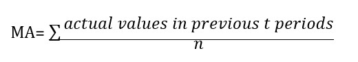
Moving Average Calculation

The Moving Averarge (MA model, proposed by G. Walker, in 1931) calculation has the role of smoothing the fluctuations of the series over time (Balakrishnan N.R., et. al., 2017) and measuring seasonal variations (Cărbunaru B., Băcescu C., 2013).

The calculation formula is represented by the average of the 12 months:

Centered moving average calculation

Taking into consideration that our series has an even number of data, we need further to calculate the Centered Moving Average if we had an odd number, wich was no longer necessary (Balakrishnan N.R., et. al., 2017). The calculation method is represented by the arithmetic mean for the successive pairs of moving averages.

Fig. 3:  Historical data and their trend obtained after the calculation of the Centered Moving Average

(Source: author’s processing in Microsoft Excel)

Seasonality and Irregularity Index

In the next step, we will extract the seasonal and the random component, dividing the data of the original series (means the realized volumes) by the centered moving average.

Seasonality Index

We will further calculate the Seasonal Index for each month and each year as an average of the previously calculated indices for each month of each year as follows.

A Seasonality Index with a value 1 indicates that volumes are above average (Balakrishnan N.R, et. al, 2017).

Deseazonalised Data

Now we will perform the deseasonalization of the data, this means that we will eliminate the influence of seasonality by dividing the original data (the sold volumes) by the seasonal index (Cărbunaru B., Băcescu C., 2013) for each month and each year.

Linear Equation Regression (Y=a+bX)

Now we need to calculate the trend of the series for a specific time frame with the help of a  simple linear regression equation, given below (Caraiani C. et. Al., 2010):

Y = a + bX, where,

– X = the time variable, independent;

– Y = the dependent variable,  that is going to be predicted;

– a = the intercept parameter;

– b = slope parameter.

We also want to point out that it is important to remove seasonal effects from the data before obtaining the trend line via the regression, otherwise, the presence of seasonal variations may affect the linear equation (Balakrishnan N.R., et. al, 2017).

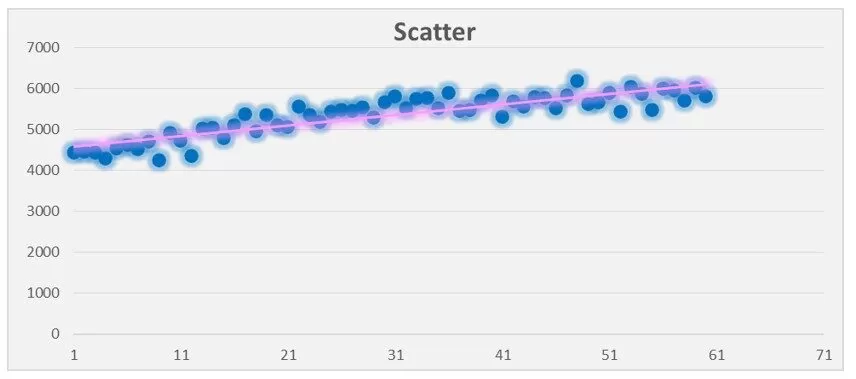
To get an idea of whether or not there is a relationship between the 2 variables, the Scatter diagram can be very useful. On the horizontal axis X, we will find the independent variable, and on the vertical axis Y, we will find the dependent variable. As it is shown in picture  no. 4, we can observe that beetween the 2 variables there is a positive relation (r= 0,87).

Fig. 4: Scatter Graph 

(Source: author’s processing in Microsoft Excel)

Trend component (linear ecuation for each period)

We will calculate now for the next year the future trend of the series, for each month, as following the example:

Y=a+b*1, for the first month – year 2023

Y=a+b*2, for the second month – year 2023

Y=a+b*3, for the third month –  year 2023

……..

Forecast (Trend*Seasonality Index)

By using the Seasonal Index, we can adjust the volumes for each quarter and year (Balakrishnan N.R., et. al.,2017). So, in order to forecast the volumes destined for the future sales, we will multiply the seasonality index with the trend as follows:

Forecast= Seasonalized Index * Trend

Results

As research results, the prediction figures we obtained (the future demands) using the time series model can further be added in the sales volumes budget for the next years. The volumes are multiplied after with the plan price calculated previously and we will obtain the revenues budget.

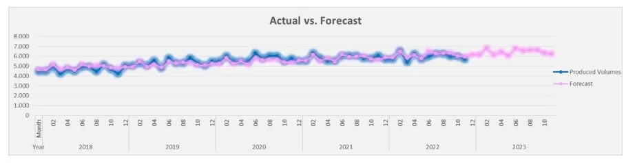
In picture no. 5, we can see ilustrated the forecast, the initial series data and the trend. We can observe how smooth the forecast line is compared to the sold volumes line. The model kept the trend that follows an increasing in volumes to be sold in the following years.

These predictions will certaintly to the management (called bottom-up approach) that will evaluate and analyze, and can see now in the present how the future looks like for the company. As we can see from the forecast, sales are increasing from one year to another so management can start and make plans, change strategies, make adjustments and take decisions like future investments for new products, production lines, market development.

Fig. 5:  Forecasted sales volumes. 

 (Source: author’s processing in Microsoft Excel)

Error metrics

In order to measure the accuracy of the forecasts, we can use the Mean Absolute Percentage Error (MAPE), which is widely used in practice (Sagaert Y. R., et. al, 2017):

where,

Yt+h is the actual sales and Y’t+h is the forecast.

More precisely, we will calculate and compare the accuracy of the predictions, this means we will measure the quality of the forecast model in comparison with the actual figures (Sohrabpour V., et. al., 2021).

The MAPE indicator shows how far the forecast deviates from the current data. Based on our realised sold volumes and forecasted ones the calculated overall average error is 0,29%, means that in avearge, the forecast deviates from the initial data with 0,29%.

Conclusions

The motive of this paper was to implement a forecasting model of the future demands through the statistical time series method, that can further be added in the sales volumes budget for the next years.

We presented the purpose of forcasting as a financial projection of the future (Laval V., 2018), types of forecasting splitted in causal model, critical model and chronological series model (Jain L. D. C., Malehorn J., 2006).

We focused then on the time series model and defined it as value of a certain type arranged in chronological order (Wang R., et. a.,  2021). We also highlited the four components of this model wich are: the trend (the upward or downward movement of data over time), the seasonality (can occur at certain intervals of time within a year), cyclical variation (are patterns that appear over several years)  and irregular component (caused by unforeseen events), (Balakrishnan N.R., et. al., 2017). In the modelling process, we firstly  have isolated  all these components, named also decomposition process, deseazonalised the data and then forecast the future sales by combining the component back in the model.

Short evolutions of the time series techniques were illustrated from the Autoregressive method (AR) where we can use the previous variable data to predict the performance of the next period, to Moving Averages (MA) method, which is a hybrid model based on the AR, known also as ARMA model.

In the methodology we presented  all the processes of modelling, starting with the analysis of the primary data that were collected via an enterprise resourse planning (ERP) system from the actual revenues budgets, from the five past years, from a company in the glass mould manufacturing area. The research framework started with  the analysis of the historical data, where we observed the seasonality, the trend, and no random component in the series. We moved forward to calculate the Moving Average and the Centered Moving Average in order to smooth the fluctuations of series over time (Balakrishnan N.R., et. al, 2017). We  extracted then the Irregularity Index and the Seasonality Index in order to perform further the deaseazonalisation of the data. Based on these data, we managed then to calculate the Linear Equation Regression needed to obtain the future trend. Finally we used the multiplicative model in order to obtain the forecast by multiplying the seasonality to the trend.

As results, we obtained the data and  the future demands, that can be added in the budgets for the next years of planning. By analysing the forecasted series, we noticed that the model kept the trend that follows an increase in volumes in the following years. The volumes that we managed to forecast will be multiplied with the plan prices and in this way we can get the budget revenues.

As a conclusion, based on the data that we could  access, the time series model was the one that could fit the best. These future predictions are very important for the management, as they can see now in the present how the future looks like and help take decisions.

The main limitation of the paper was the access to the information, which means we only used the sales budget from just one company, as in the management accounting field it is quite hard to have real data about the whole business.

Future Research

This paper presented the forecasting technique done via the time series model, but beside this one, as we saw in the litterature review, there are still many other models and methods we can use when we want to see future trends. Certainly, we always have to analyse and see what kind of data we have and what kind of variables the model has.

When coming to predict sales budgets beside the time series univariate model, that uses as dependent variable information from the microeconomic field, we can also use other variables that can influence sales, as the marketing mix factors (Sohrabpour V., et. al.,  2021). We can also use data coming from the macroeconomic domain, that can certainly affect the sales of the company, when we operate in an unstable economy and market.

Either for the marketing mix or for the macroeconomic data, we can use the causal forecasting model where there is a  relationship between a set of dependent and  independent variables (Sohrabpour V., et. al., 2021).

The difference between traditional time series and causal methods is highlighted when sales behavior changes in an unstable pattern, and there are apparently unpredictable fluctuations in its trend. This happens in unstable economies or in markets in which economic factors affect sales behavior in a complex manner. To be able to forecast future sales in such circumstances, merely relying on historical time series techniques is not useful. Thus, causal forecasting methods capable of identifying the relationships between variables in a sales model are used to determine future sales behavior.

References

• Anghelache C., Manole A., Seriile dinamice / cronologice (de timp) – prezentare teoretică, structură, relaţiile dintre indici, Romanian Statistical Review no. 10, 2012
• Balakrishnan N. R., Render B., Stair M. R., Munson C., Managerial Decision Modeling, Ed. Walter de Gruyter Inc., 2017, Berlin
• Caraiani C., Dumitrana M., Control de Gestiune, Ed. Universitară, 2010, București – Fan Z. P., Che Y-J., Chen Z-Y., Product sales forecasting using online reviews and historical sales data: A method combining the Bass model and sentiment analysis, Journal of Business Research 74 (2017) 90–100
• Cărbunaru A. B., Băcescu Condruz M., Metode utilizate în analiza variaţiilor sezoniere a seriilor cronologice, Revista Română de statistică, mr. 3, 2013
• Gao J., Xie Y., Cui X., Yu H., Gu F., (2018) Chinese automobile sales forecasting using economic indicators and typical domestic brand automobile sales data: a method based on econometric model, Advances in Mechanical Engineering, 2018, Vol. 10(2) 1–11
• Gonçalves J.N.C., Cortez P., M. Carvalho S., Frazao N. M., , A multivariate approach for multi-step demand forecasting in assembly industries: Empirical evidence from an automotive supply chain, Decision Support Systems 142, 2021
• Hannagan T. J., Mastering Statistics, Macmillian Education LTD, 1991, London
• Ivert K., D-P. I., Kaipia R., Fredriksson A., Dreyer C. H., Johansson I. M., Lukas Chabada, Cecilie Maria Damgaard & Nina Tuomikangas, Sales and operations planning: responding to the needs of industrial food producers, Production Planning & Control: The Management of Operations, 2014
• Jain L. D. C, Malehorn J., Benchmarking: Forecasting Practices: A Guide to Improving Forecasting Performance, Ed. Graceway Publishing Company, NW, 2006
• Laval V., How to Increase the Value-added of Controlling, 2018, Berlin
• Lawrence M., O’Connor M., Edmundson B., A feld study of sales forecasting accuracy and processes, European Journal of Operational Research 122, 2000
• Marshall P., Dockendorff M., Ibanez S., A forecasting system for movie attendance, Journal of Business Research 66 (2013) 1800–1806
• Sagaert Y.R., Aghezzaf EL-H., Kourentzes N., Desmet B., Tactical sales forecasting using a very large set of macroeconomic indicators, European Journal of Operational Research, 2017
• Sagaert Y.R., Kourentzes N., De Vuyst S., Aghezzaf E.-H., Desmet B., Incorporating macroeconomic leading indicators in tactical capacity planning, International Journal of Production Economics, 2018, 12–19
• Sarfo P.A., Mai Q., Sanfilippo M. F., Preen B. D., Stewart L. M., Fatovich D. M., A comparison of multivariate and univariate time series approaches tomodelling and forecasting emergency department demand in Western Australia, Journal of Biomedical Informatics 57 (2015) 62–73
• Seval E., Nursel O., Grey modelling based forecasting system for return flow of end-of-life vehicles, Technological Forecasting & Social Change 115 (2017) 155–166
• Sohrabpour V., Oghazi P., Toorajipour R., Nazarpour A., Export sales forecasting using artificial intelligence, Technological Forecasting & Social Change 163, 2021
• Thanh-Lam N., Shu M-H., Huang Y-F., & Hsu B-M., (2013) Accurate forecasting models in predicting the inbound tourism demand in Vietnam, Journal of Statistics and Management Systems, 16:1, 25-43
• Wang R., Pei X., Zhu J., Zhang Z., Huang X., Zhai J., Zhang F., Multivariable time series forecasting using model fusion, Information Sciences 585, 2022, 262–274
• Zhang C., Yu-Xin Tian, Fan Z-P., Liu Y., Fan L-W., Product sales forecasting using macroeconomic indicators and online reviews: a method combining prospect theory and sentiment analysis, Springer-Verlag GmbH Germany, part of Springer Nature, 2019.