Squeezing the Curve: Unlocking Yield Information for Better Recession Forecasts in the CEE Region

Introduction

The yield curve inversion has often been considered in the literature as the most important early warning signal of a recession. It is generally accepted in the literature that the yield curve inversion has informational power about the onset of an economic downturn, but only if the inversion is persistent over time. Particularly in the recent period, marked by multiple economic and social crises, inverted yield curves have been observable (e.g. for the yield curve of US Treasury securities), but for truly short periods of time. These inversions have not been followed by negative developments. Therefore, an inversion of the yield curve is considered to be an early warning if the inverted shape persists for at least 2 or even 3 quarters.

The inversion of the yield curve implies higher yield to maturity for the bond with the shortest existing maturity than for the one with the longest maturities. This situation, in normal times, might be considered counter-intuitive economically. Under normal circumstances, in order to respect the time value of money principle, the bond with higher tenor should offer a higher yield. However, in the run-up to economic crises, the inversion implies lower investor confidence in the issuer and its credit risk suitability over shorter maturities, due to the probable negative effects of crises on the issuer’s ability to repay.

For many countries during the Great Financial Crisis, the inversion of the yield curve indicated the onset of a recession. The question arises, however, whether the inversion of the curve could still have informative power today. In the literature, the effects of quantitative easing on the yield curve were very much discussed and some results indicated that the upward slope permanently declined. Another significant question is in fact if the yield curve could have information about more focused concerns, like the industrial production which is considered a good proxy for the aggregate activity. Now the industrial production in the European Union seems to be weakened and therefore the yield should tell something about this.

A major vulnerability nowadays in the European Union’s economy is the industrial sector, which is in a recessionary phase in many countries like Romania, according to analysts. Romania’s industrial production index has been declining since 2019, with the downturn intensifying in the last year. Structural and cyclical factors, such as poor diversified industry and the Germany’s economic slowdown, have impacted Romania, as Germany is the destination for around 20% of Romania’s exports, mostly industrial goods (poor diversified activities). Also, Romania’s currency has remained stable since the pandemic, indicating overvaluation, and its industry relies on low value-added activities, making it less competitive, especially with rising wages. This paper examines whether the yield curve could signal these economic trends and their impact on industrial output. We believe that the yield curve’s predictive power for Romania has weakened recently and may no longer reliably forecast industrial turning points.

Literature

Estrella and Hardouvelis (1989) is a seminal paper highlighting the yield curve as an early warning indicator for recessions. The paper shows that a positive curve slope signals future economic growth, improving predictions over other indicators such as lagged economic growth and inter-bank interest rates. Also, they find that average quarterly yields provide better statistical significance than end-of-quarter yields.

Mehl (2006) examined the interaction between the yield curve and industrial output in emerging economies, focusing on the Czech Republic, Hungary, and Poland—peers of Romania. Panel linear regression was employed and term spreads from the US and EA have been used as regressors to highlight spillover effects. Results indicated that the yield curve slope improves economic forecasts over short and even long horizons, with significant spillover effects noted.

Backer et al. (2019) judge the yield curve to be similar to Princess Cassandra of Troy, who predicted the fall of her city. The authors compare multiple studies and discuss the implications of contemporary business cycles and unconventional monetary policies on predictive power, suggesting that predictive power has improved over time. The paper concludes that although there have been a number of structural changes over time, the shape of the term structure still needs to be considered, but it really needs to have an inverted persistent shape.

Grab and Titzck (2020) argued that recession probability is overestimated, as Backer et al. (2019) noted a shift in the economic-financial paradigm, highlighting that in 2019, when the term structure slope was low, many economists predicted a recession. This is due to the influence of quantitative easing (QE) programmes of ECB and Fed, as well as spillover effects from other central banks engaging in substantial security purchases. They suggested that the slope of the curve has artificially declined over time. To address this, they proposed adjusting the term spread to account for factors like US QE programs and ECB actions. Adjustments lowered recession probabilities, especially when all factors were included. This paper emphasizes that an unadjusted term spread could lead to numerous false alarms, type 2 errors, regarding recession predictions.

Haubrich (2021) conducts a review of the literature on yield curve inversion and recessionary periods. It is concluded that in the post-World War II period the yield curve had significant predictive power, but still differed from period to period, depending on the economic events at the time or the political mandates in the US. The authors suggest that for the United States the results were often more satisfactory, but still the yield curve remains relevant for countries such as the UK or Germany. Haubrich (2021) provides evidence (through previous studies) on the fact that the time aggregation of yield curve and yield convention data can significantly skew results and even ultimately lead to false positive events.

Sabes and Sahuc (2022) examine the yield curve’s predictive power for Euro area countries from 1970 to 2022, finding that curve inversion remains informative primarily for core countries. For others, predictive capacity is impacted by credit risk premiums. Analysing two samples (1970-2022 and 1970-2008), they show a significant increase in predictive power, with the AUROC rising from 0.75 to 0.92 for the latter, suggesting a decrease of performance during the last decade. Individual analyses reveal that France, Italy, and Spain have AUROC values below 0.7, indicating they are perceived as riskier compared to the German Bund, which complicates the relationship between economic developments and the term structure.

Eser et al. (2023), on a much more rigorous note and strictly focused on the recent period, validate that quantitative easing programs at least had an impact on the yield curve for the Euro area. Thus, the hypotheses specified by Backer et al. (2019) and Grab and Titzck (2020) are validated; there are noises in the information provided by yield curves.

Fonseca et al. (2023) consider the evidence indicated by Eser et al. (2023) and discuss the signals indicated by the yield curves for the Euro Area and the US in recent years. In the absence of using other indicators, such as the CISS and excess bond premium (for the US) or the CISS (for the Euro Area), the probability is overestimated. The term spread decomposition is also discussed and suggests that the evidence from previous literature holds true. When the inversion of the curve is due to the inversion of the real curve rather than to market-based inflation compensation, then the yield curve information regarding economic outlook is lower.

Bussier and Lhuissier (2024) discuss the predictive ability of the yield curve inversion for recessionary periods in the euro area. The authors argue, in a similar vein to the findings of Sabes and Sahuc (2022), that the predictive performance has decreased in the post-Great Financial Crisis period as a result of the quantitative easing programmes implemented. Bussier and Lhuissier (2024) estimate Probit models for the time horizon 1970-2009. Then they perform an out-of-sample evaluation for November 2023, when the inversion of the euro area yield curve happened. Using a probability threshold (obtained by maximising the ratio TP to FP), the authors show that the probability is overestimated and generates a false signal. In-sample, there is moderate accuracy using the slope of the yield curve.

Data and Methodology

A study for Romania is rather difficult to carry out, as few statistical records are available. On the basis of existing government issues, the yield curve for Romania was only formed in the second half of 2007. The lowest maturity is 6 months and the highest is 10 years. A solution to improve the estimations in the context of a medium sample is the Bayesian inference. Data regarding the term spread have been used in level, in difference (year on year), but also as a categorical variable that reflects the persistence of negative growth rates of the industrial production.

Typically, logistic regression is used to estimate the probability of negative industrial production growth based on the term spread lags. However, we argue that relying solely on the recent term spread or its previous evolution is insufficient. Early movements, such as year-on-year term spread dynamics, must be considered alongside a recently spread state. Additionally, the persistence of yield curve inversion increases recession probability. To capture this, we created a categorical variable ranging from one to nine, counting the number of consecutive months of term spread decline. Also, we transformed the variable in the exponential form. We capped the index at nine months, as such a period is sufficient, considering the rule of thumb of 2-3 quarters of inversion, but also to avoid underestimating short-term changes while using the exponential form.

Each multivariate model has three variables, beyond the intercept: lag of the term spread, lag of the year-on-year term spread change and one of the two persistence indicators (either the normal or the exponential form). To avoid multicollinearity, a mix of closer-term spread and further lags of year-on-year changes is necessary, as using similar lag numbers for these variables would compromise the model’s reliability. The following abbreviations will be used in the article:

Table 1: Variables legend

The data sample spans August 2008 to July 2023, comprising 180 monthly observations sourced from Refinitiv Eikon and the Romanian National Statistical Institute. Following Estrella and Hardouvelis (1989), the monthly yield to maturity for the term spread was calculated using daily averages rather than the yield in the last day of each month.

The correlations between the candidate regressors and the binary dependent variable (1 for a negative year on year evolution of the industrial production index, 0 for a positive evolution) were initially studied and the target was to achieve correlations as high as possible.

The second and the third lag of the term spread were indicating the highest correlation with the state variable, among the lags of the term spread. Also, the seventh lag has a comparable correlation coefficient, even though it is counter intuitive with the gradual diminishing importance. Still, the univariate model with the seventh lag has been checked. It is noticeable that using more than one lag of the term spread in a multivariate setting is not suitable, due to the remarkably high autocorrelation, which indeed had been expected due to inertia that economic variables possess.

Table 2: Correlation matrix between term spread lags and binary variable

Seventh, eighth, and ninth lags of the annual term spread dynamics are showing the highest correlations with the binary variable, the ninth lag exceeding -0.4. It seems that the dynamics registered a long time ago have a stronger relationship than the more recent term spread values.

Table 3: Correlation matrix between lags of term spread year-on-year changes and binary variable

Then, to avoid multicollinearity, the presence of low correlations between the potential regressors was sought. There is a low correlation precisely for the lags of the term spread closer to the present with further back in time lags of the change in the term spread (as an example, the second lag of the term spread in combination with the seventh lag of the dynamics represents a good mix).

Table 4: Correlation matrix between lags of changes in term spread and lags of the term spread

Based on the correlation analysis, to achieve an explanatory power as high as possible but with a minimum correlation between regressors, the following multivariate configurations had been tested.

Table 5. Multivariate candidate models

To address the research problem, we employed two classical classification models: Logit and Probit. The estimation utilized Bayesian inference with diffuse or informative prior distributions for each regression coefficient. We estimated the regressions using Markov Chain Monte Carlo (MCMC) simulations, running fifty thousand iterations to ensure coefficient convergence, applying a burn-in of five thousand simulations (10% of total iterations). In logistic models, coefficients followed normal prior distributions. However, for the Probit model, the normal distribution proved inadequate for the variable indicating negative change persistence, leading to convergence issues and autocorrelation among coefficients. Therefore, we used a log-normal distribution for this coefficient, also considering that intuitively it should take positive values. The Deviation Information Criterion (DIC) was the main measure of fit due to the Bayesian approach, with Log-Pseudo Marginal Likelihood and Bayes Factor, employed to compare models with similar DIC.

The earlier mentioned multivariate models were estimated using logistic regression with diffuse priors. Two models stood out in terms of performance. After identifying the best two configurations with logistic regression, we also estimated these models using the Probit model. Next, we estimated the top two configurations with both Logit and Probit models, but applying informative priors for term spread changes. Typically, we specified only one informative prior to avoid bias. In some cases, also for the term spread lags when coefficients were insignificant with diffuse priors.

The models were compared using LPML and Bayes Factor. But we still did not offer a complete view regarding our research question, whether the yield curve characteristics have good predictive power regarding the reversal of economic cycles or not. As a final analysis, the area under the ROC curve was checked. As a back testing, we analysed the out of sample performance during August 2023 – August 2024. It was intended to perform an “acid” test of performance using the available sample of data from August 2023 to August 2024. The out-of-sample evaluation contains a small number of observations, only 13, from which 9 observations include negative dynamics of the industrial production index. Under such conditions it was expected that the model using strictly yield curve information would perform worse than in-sample. But the question is: how low is the performance under such circumstances?

Results

Univariate models with diffuse priors (LOGIT models)

In the univariate analysis we observed that the term spread, in its classical form, gives, regardless of the lag, a lower fit than the lags of the dynamics and the indicators of persistence in decline. The third lag of the term spread gives a slightly better fit than the second lag. The 9th lag of the term spread dynamics is significantly better at explaining the available data on the state of the economy than the remaining lags of the dynamics. Although there were higher expectations about the difference of the two persistence indicators, the differences are insignificant, at least in the univariate analysis and we cannot say that the exponential form boosts the performance.

Table 6. Univariate models with non-informative prior

Significance: ** significant coefficient at 5% level, * significant coefficient at 10% level

Multivariate Analysis

The signs of the obtained coefficients in the univariate models exhibit the economic intuition. Regardless of the lag, the term spread exhibits a negative coefficient. So, as the maturity spread is smaller, there is a higher probability that the industrial production index exhibits negative dynamics. The coefficient on the year-on-year change in the term spread is also negative irrespective of the lag used and the model. With a negative change in the term spread, economic developments are more likely to decline. Importantly, the variables count_ts9 and e_count_ts9 are always significant at a 5% confidence level and show that as more consecutive months of negative term spread change arise, the probability of a recession increases, even exponentially.

Looking at the multivariate results, the 9th lag of the term spread change offers an improvement in Deviance Information Criteria value. In terms of the term spread, we cannot identify very clearly whether the second lag performs better than the third in a multivariate combination. Three models show a DIC between 175 and 178, two models a DIC above 179, and two models differ quite strongly from the rest in terms of DIC value, which is 172.7 (for both). The latter two models have the exponential persistence indicator of the change in term spread and use the 9th lag of the change in term spread, the difference between the two being the lag of the term spread used, the second or the third. However, the coefficients are similar.

Thus, we have two models that differ from the rest and between them there is a high competition. It is worth noting, however, that the lag of the term spread for both models is not statistically significant even at the 10% level, which might suggest that the term spread could be eliminated among the regressors. The other models with lower DIC values mostly have all regressors statistically significant at least for a 10% level. We strongly believe that the term spread lags significance could be enhanced using Bayesian inference through informative priors. I think the most critical point to highlight from these logit models is that persistence matters, validating the rule of thumb, and as there are several consecutive declines in the term spread, the probability of an economic decline is increasing, but the relationship might be nonlinear, even exponential.

Table 8. Multivariate Logit models with non-informative priorsSignificance: ** significant coefficient at 5% level, * significant coefficient at 10% level

As an additional way of modelling, the two best obtained configurations were also estimated as Probit models. We initially ran them using the previous assumptions. The coefficients follow non-informative normal distributions of mean 0 and precision 0.01. Fifty thousand simulations were run, of which the first 5000 were excluded from the sample. For these hypotheses, we observed convergence problems for the coefficient of e_count_ts9 using the simulation history, and autocorrelation problems for all coefficients. Therefore, the basic assumptions have been modified. We assumed for all the coefficients the same type of distribution, non-informative normal, apart from the e_count_ts9 coefficient. For the coefficient of the last variable, we assumed an a priori log-normal distribution (since the positive value of the coefficient was generally accepted by all configurations and it is intuitively economical that it takes positive values). A thin option value of 10 was used in MCMC to reduce the autocorrelation of the coefficients.

With the new priors, the problems had been solved. Historically, the coefficients converged and showed the absence of autocorrelation. Coefficients on quantiles do not show large deviations.

Using the Probit model, we observe that for both configurations all coefficients are statistically significant at least for a 10% significance threshold. Configuration 1 shows all coefficients statistically significant for 5%, an exception is the coefficient for L2_TS. However, for the second configuration, 3 out of 4 coefficients are only significant at 10%, not at 5%, and therefore the model should be used with caution or simultaneously with the other model in order to have an alternative prediction. Importantly, in contrast to the LOGIT models, DIC is much lower as all coefficients become statistically significant, which shows us a better performance by Probit.

Table 9. Multivariate Probit models with non-informative priorsSignificance: ** significant coefficient at 5% level, * significant coefficient at 10% level

Multivariate analysis using informative priors

In the univariate analysis, the 9th lag of the term spread showed a much better fit than other variables, prompting us to impose informative a priori distributions for its coefficient in the multivariate models (to boost the performance). We also applied informative priors in the logit models to the lags of term spread, in the idea of improving its significance. We used the median values from the univariate configurations.

It can be said that these Bayesian estimates with a priori informative distributions brought significant improvements to the configurations through both Logit and Probit. In the Logit models, all coefficients become statistically significant even for 5%, and the DIC values are lower even than those of the previously obtained PROBIT models with non-informative distributions of coefficients. Logit configuration 1 registers a massive improvement on the informational criterion. However, even better performance is reached using informative distributions for the coefficient of L9_D_TS, in the case of the Probit models compared to Logit. The Probit models again climb the podium in terms of DIC values.

Table 10. Multivariate models with informative priorsSignificance: ** significant coefficient at 5% level, * significant coefficient at 10% level

The difference is not exceedingly high between the two Probit models (163.4 vs 163.9). Therefore, we decided to study the performance of the two, by alternative criteria, Bayes Factor computed by means of marginal likelihood functions and by comparing LPML functions.

Results obtained do not support the hypothesis that configuration 1 is significantly better than configuration 8, for Probit with a priori informative distributions. A Bayes Factor of 1.07 was obtained, which, according to the grid proposed by Raftery (1996), falls within the range of values with weak evidence (values between 1-3) for the superiority of configuration 1. The Pseudo-Log Marginal Likelihood for configuration 8 even has a higher value than that for the first configuration, indicating rather that the alternative model is better. Thus, we cannot consider that there are significant differences between the two models and rather they could be used simultaneously.

Table 11. Bayes Factor and LPML

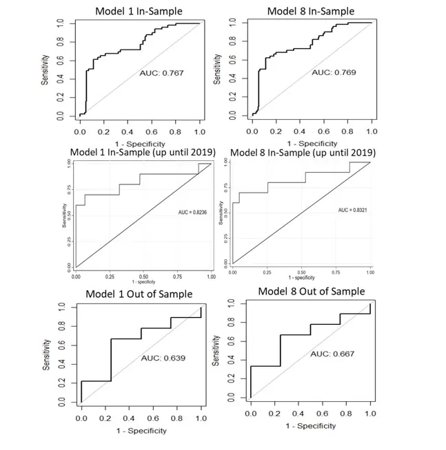
From a predictive ability perspective, AUROC values were analysed, with both models exceeding the 0.7 threshold, achieving 76% under the ROC curve, indicating decent in-sample classification performance. Interestingly, when using December 2018 as the last observation, the AUROC for both Probit models rose above 80%, having values of 82% and 83%. This suggests that the yield curve’s predictive power weakened after 2019, when the industrial production started a persistent downward path. Out of sample (August 2023-August 2024) performance declined, with AUROC values of 0.63 and just above 0.65 for the models. The small and unbalanced dataset likely hindered performance; a larger more balanced dataset might yield better results. While incorporating a lag of industrial production could enhance predictions, this study aimed to isolate the term spread’s interaction with industrial production. Thus, introducing additional indicators would have compromised objectivity. Despite the modest performance, the eighth configuration could still be relevant when combined with a persistence indicator or Germany’s economic outlook.

Fig 1. Area under the ROC curve

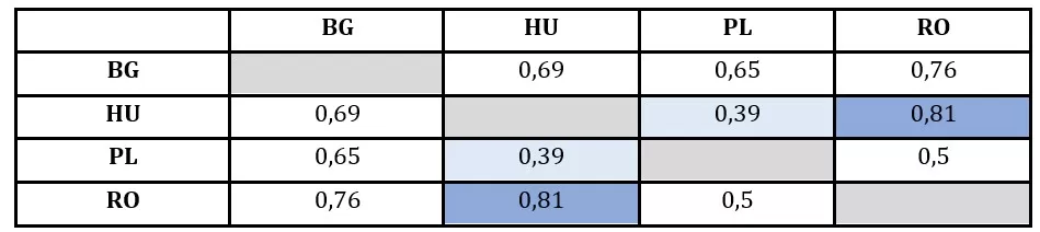
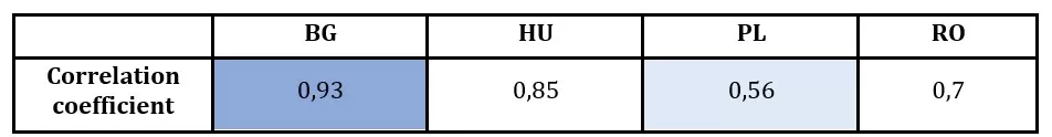
A brief analysis was also conducted for other economies in the Central and Eastern European region. The Czech Republic, Poland, and Hungary were chosen as they are often seen as reference countries for Romania in macroeconomic analysis. Logistic regression models, estimated by classical statistical inference, were performed, having as regressor only the term spread used with a certain number of lags, similar as for Romania up to 9 lags (3 quarters).  The main objective is to check whether the decrease in prediction performance is available just for Romania or for other countries from the CEE as well.

First, as a brief remark for Poland and the Czech Republic, an increasing performance is observable as the forecast horizon is wider. Thus, for these countries, early warning at a relatively medium time horizon of about 2-3 quarters is indicated, which is in line with the heuristic prediction rule using yield curves. In the case of Hungary, AUROC values remain above 70%, even above 75% for any horizon, and this better performance does not differ much by horizon as it happens for the other two countries.

As for the final purpose of this analysis, the hypothesis that since the outbreak of the pandemic there has been a period of inhibition of the link between industrial activity and yield curves at the regional level, not only at the Romanian level, is partially accepted. In the case of the Czech Republic, performance for the pre-Covid-19 sample is higher on average by even 5 percentage points of AUROC. For Hungary, similarly, performance is on average 3 percentage points higher in AUROC terms, compared to the full sample accuracy. Only in the case of Poland, the full sample estimates seem to perform better. However, it is important to note that for only 4 lags out of 9, the AUROC values for Poland are significantly higher than the 70% threshold. Therefore, the case of Poland should be treated with caution, as we cannot distinguish a clear relationship between industrial and yield curve developments in any sample.

Thus, we can conclude that what we have observed for Romania is not a particular phenomenon. It is common to other economies in the region. There is a decoupling tendency, as the curve most likely reflects financial market expectations about other components of the economy most likely nowadays.

Now having the performance of very simple yield curve models for Romania, we see that the information offered simply by the yield curve without advanced modelling is not sufficient. Initial estimates with multiple yield curve derived indicators and Bayesian inference offer even higher performance than the simple models applied for the pre-covid sample. The AUROC difference is over 9 percentage points for almost all the cases.

Table 12. AUROC values for Logit-Early Warning Models for the CEE region

Conclusions

To summarize, we can say that the term spread is indeed an indicator with moderate capacity of predicting industrial developments, even for an economy like Romania, as long as the shifts in the yield curve are persistent. However, it is quite reasonable to judge the results as a sign of weakening of the relationship. We have seen that for the out of sample robustness check with numerous episodes of negative industrial production dynamics, the AUROC for the two models does not exceed 0.7. Also, the AUROC is higher when using a smaller sample that excludes the negative trend started by the industrial production in 2019. In this regard, not only the yield curves from the Euro Area faces a diminishing predictive power, as suggested in the literature, but also the ones from European Union members. Romania is not a particular case of the CEE region.

In this regard, we do not propose to eliminate the yield curve from the potential list of predictors, but certainly nowadays if estimating the state of industry is the desired objective, one should check also for other factors. For example, in the case of Romania, probably a proxy for the Germany’s activity would be suitable. Contrary to Backer et al.’s (2019) metaphor linking the yield curve with the Cassandra Princess, we suggest that the yield curve should not be seen as a witch with a crystal ball.

This paper has shown that simultaneously relying on information regarding a recent state of the yield curve, historical dynamics and regarding the persistence of negative dynamics, could provide moderate information about the probability of an industrial recession. The addition of a persistence indicator, even with an exponential form, brings improvements. But the recent period has a large number of false negative errors. We have seen that by implying informative prior, the results could be enhanced and the Probit models perform better. Finally, the limited literature and datasets on this subject for the CEE region, indeed, requires Bayesian methods. Compared with simple models that use the yield curve, our methodology significantly outperforms them.

Finally, this paper shows that Romania is not the only CEE economy for which yield curve information is of decreasing importance. Also, for the Czech Republic and Poland, the models that include Covid-19 and post-Covid-19 data are less efficient in early warning than those using only the pre-Covid sample. Thus, the proposed Bayesian estimation strategy could be helpful for practitioners interested in early warning industrial recession in other CEE countries as well.

Bibliography

• Backer, B., Deroose, M. and Nieuwenhuyze, C. (2019), `Is a recession imminent? The signal of the yield curve`, NBB Economic Review June/2019.
• Bussiere, M. and Lhuissier, S. (2024), `What does an inversion of the yield curve tell us?`, Bulletin de la Banque de France, 250(3).
• Eser, F., Lemke, W., Nyhom, K., Radde S. and Vladu, A.L. (2023), `Tracing the impact of the ECB’s asset purchase program on the yield curve`, International Journal of Central Banking, 19(3), 359-422.
• Estrella, A. and Hardouvelis, G. A. (1989), `The term structure as a predictor of real economic activity`, FRBNY Working Papers, WP 7/1989.
• Fonsenca, L., McQuade, P., Van Robays, I. and Vladu, A.L. (2023), `The inversion of the yield curve and its information content in the euro area and the United States`, ECB Economic Bulletins, ECB Economic Bulletin, 7/2023, 42-46.
• Grab, J. and Titzck, S. (2020), `US yield curve inversion and financial market signals of recession`, ECB Economic Bulletins, 1/2020, 25-28.
• Haubrich, J.G. (2021), `Does the yield curve predict output?` , Annual Review of Financial Economics, 13/2021, 341-62.
• Mehl, A. (2006), `The yield curve as a predictor and emerging economies`, ECB Working Papers, ECB WP Series 691/2006.
• Raftery, A.E. (1996), `Approximate Bayes factors and accounting for model uncertainty in generalised linear models`, Biometrika, 83/2/1996, 251–266.
• Sabes D., J.G. Sahuc (2022), Do yield curve inversions predict recessions in the euro area, Finance Research Letters, 52(C).