Faculty Development Program Alumnus, University of North Florida
Faculty of Economics and Finance, Saint-Petersburg State University of Economics, Sadovaya, St. Petersburg, Russia
Volume 2018,
Article ID 684518,
Journal of Economics Studies and Research,
26 pages,
DOI: 10.5171/2018.684518
Received date: 8 February 2018; Accepted date: 30 May 2018; Published date: 31 October 2018
Academic Editor: Liudmila Nikolova
Cite this Article as:
Konstantin B. Kostin (2018), “Global Companies’ Growth Potential Assessment via Application of Economic Cycles", Journal of Economics Studies and Research, Vol. 2018 (2018), Article ID 684518, DOI: 10.5171/2018.684518
The purpose of this article is to investigate different economic cycles and their application to the modern international business environment and more specifically the growth potential assessment of global companies. Within the framework of the analysis, the cycle theories were classified into short-term and long term. Their applicability to forecasting different economic factors such as interest rates, inflation rate and the general state of the economy as well as investment attractiveness and growth potential of various asset classes, was investigated. The special framework was developed to assess the investment attractiveness and growth potential of various stocks. Three asset classes from the hospitality industry (the total of 15 stocks) were selected for the proposed framework application in order to determine the stocks with the highest investment attractiveness and growth potential. The obtained results are presented in the article.
Keywords: economic cycles, international business, economic growth, economic forecast.
Introduction
The economic cycle is an important instrument to analyze past, current and future international business activities around the world as it opens forecasting opportunities if one can interpret it. Economic cycles are the first option the economist could utilize to access how well the economy under investigation is operating at a specific point in time. Factors such as gross domestic product (GDP), interest rates, levels of employment and consumer spending can help determine the current stage of the economic cycle. The ups and downs correlate with the unemployment rate, inflation and future expectations of market participants. This offers ample information on how financial institutions should react to the market situation.
Each economic cycle consists of four different phases. The stages include expansion, peak, contraction and trough. The stages differ in length and can somewhat vary from cycle to cycle. When the economy overheats, the cycle reaches its peak and drops down afterwards. The economy is starting a recession with higher unemployment rates and negative or small GDP growth. After that the trough phase starts and the economy adapts, and growth diminishes. After that the expansion phase starts again. By studying different economic cycles, the reasons for special developments could be detected. These reasons can be analyzed and used for practical business applications and forecasting. It is important to deal with the economic cycles in different countries using the right reference points or a certain timeframe to observe whether there is a correlation and whether events follow each other with a certain delay. The economic cycles offer a wide spectrum of opportunities to compare countries and their productivity. By interpreting the economic cycle of a country, one can see the current situation and predict when a phase ends and another starts. This offers the opportunity not only for better business decisions from a company perspective, but also for institutions that try to keep a well running economy, like for example the federal banks (Edelson, L., 2016). In fact, to stay on track concerning recent developments sounds easier than it really is. The globalized world has different regional characteristics, but some factors influence the economies all over the world. On the one hand, to stay up to date with new developments is crucial enough, but to follow the right predictions regarding the future on the other hand is even much more important.
The economic cycle offers ample data on the current situation in various economies. Hence, different applications on how to use the economic cycle as an instrument for efficient business activities could be developed. The problem lies in the complexity and the interdependencies between the business cycles all over the world. An economist who understands the economic development can adjust the strategies according to the business cycle performance on a short-term, mid-term or a long-term basis. Individual investors and economists make their living from understanding how the economy functions and capitalizing on the market investment that results from their analysis. For this reason, many theories emerged over time in an attempt to apply logic to a seemingly emotional process. Researchers analyzed influencing factors, such as technological innovation, investment levels, the relay of information, and the laws of supply and demand, and discovered correlations regarding market developments. Considerations included not only technical factors, but also more unpredictable factors such as emotional reactions to developments and even the effect of the presidential election cycle. Despite the development of several compelling theories, the primary difficulty in understanding the complex network of modern markets lies in establishing causal relationships rather than correlative ones.
In an effort to keep the information organized and focused, the article is structured as follows. The first part defines and analyses selected long-term cycle-theories and the second part investigates selected short-term cycle theories applicable in the global environment. The theoretical findings on each theory are also supported by the analysis of potential practical theory applications for financial policy adjustments as well as for forecasting and investment strategy formulation in the international business environment. The results of Elliott Wave Theory application to investment portfolio selection from the three classes of investments from the tourism industry are presented.
Cycle Theories’ Evaluation
Paul Samuelson has described economics as “the oldest of the arts, the newest of the sciences”, when he won the Nobel Memorial Prize in Economic Sciences as the first American in 1970. The study of economic cycles, also known as business cycles, was developed during the 19th century, because economists noticed regular cyclical fluctuations in the economic development process during the British economic crisis in 1825. After this the “classical economic cycle theories” emerged. When Hayek defined the economic cycle as the circular deviation from an economic equilibrium in 1921, economists began to use this definition as the starting point of the economic cycle. Nowadays, there exist several different economic cycle theories, e.g. the classical economic cycle theory, the Keynesian or the Neoclassical School. Since all of them have their own limitations, current economists keep researching further the economic cycle theories and their applications.
Economic cycles can be defined as fluctuations in the aggregate economic activity of a country which takes place on a repeating basis over a number of months or years. In recent decades, economists have made good progress in the economic cycle studies. For a comprehensive evaluation on national economic fluctuations, it is expedient to use a comprehensive set of different indicators nowadays, such as the economic growth or the output rate to name just a few for measuring economic activity. There is currently a great combination of indicators required to evaluate economic fluctuations. The gross domestic product (GDP) growth rate, the unemployment rate and the inflation rate would also top the list of most important indicators to be evaluated. Focusing on theoretical analysis some researches have adopted an econometric method to study the causal factors of the economic cycle. Economic cycles are typically measured by considering the growth rate of real GDP, – the measure of a countries’ output. To be more precise, an economy is considered to be in recession when there are two continuous quarterly declines in GDP.
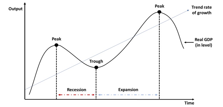
As was already mentioned in the introduction, the economic cycle consists of four stages: expansion, peak, recession and trough. The expansion phase occurs simultaneously in different economic activities. Expansions are followed by recessions, the trough and afterwards lead to new revitalizations resulting once again in an expansion phase in the next period. This system of changes repeats itself, oftentimes on an unregular basis. The fluctuations during an economic cycle can differ from more than one year up to ten or even twelve years. Generally, most expansion and recession stages last six months at least. That means that the economic cycle is far away from being a uniform, neither in amplitude nor in time periods. The proportions of cycle upswings and downswings can vary from being very minor to being devastating in every single period as shown in Figure 1.
Fig. 1: Representation of the economic cycle (Created by author based on the data acquired from Aimar, T., Bismans, F. and Diebolt, C., 2015).
These characteristics are associated with the economic cycle and its further applications. Moreover, since the world population is growing, and the technology keeps advancing from year to year, the economy displays a worldwide growth trend. Figure 1 displays how the economic performance fluctuates around the projected long-term growth trend. If we take a closer look at each of the four economic cycle phases, expansion, recession, trough and the revival, there can be several comparable features noticed in each phase. The most important features that arise during the expansion phase are e.g. a large volume of production, trade and consequently a high level of employment and job opportunities which at the same time increase a countries’ GDP. Moreover, a rising structure of interest rates can be anticipated as well as a growing volume of borrowings on the consumer and business side. As a result, investment volume grows significantly, which in turn leads to business expansion. The coherence between these developments is rather straightforward. When trade and production expand, it stimulates the demand for labor. Increased employment leads to larger wage payments which results in greater consumption which once again stimulates trade and production (Aimar, T., Bismans, F. and Diebolt, C., 2015). The properties of the recession phase are just the opposite of those of the expansion phase. The National Bureau of Economic Research classifies a recession as “a significant decline in economic activity spread across the economy, […], normally visible in real GDP, real income, employment, industrial production” (NBER, 2010). In this sense, at this stage, business optimism transforms into pessimism.
Beside the economic cycles, there are other important macroeconomic variables with cyclical properties as well, such as the GDP growth, the consumer price index, corporate profits, productivity, employment, federal budget deficit/surplus or the credit spread and more (Silvia J. E., Iqbal A., Swankoski K., Watt S., and Bullard S., 2014).
Long Term Cycle Theories
As we have already identified, the market economies are characterized by two main periods, a long-term growth trend and more or less significant short-term fluctuations in activity around this trend. In order to find an explanation to such phenomena, many economists have conducted corresponding research. As a result, they have identified and described several economic cycles which enable us to understand the logic behind economic crisis to be able to forecast their repetition in order to take measures to minimize their effects. Let us start our evaluation from the long-term cycles. A long-term cycle which is present in capitalist economies represents long-term, high-growth and low-growth economic periods. Several long-term cycle theories were selected to be presented in the next section as follows: The Austrian Business Cycle Theory, The Kondratieff Long Economic Cycles, The Elliott Wave Theory and a medium-term Juglar Cycle Theory.
The Austrian Business Cycle Theory
The Austrian Cycle Theory is largely underscored by its emphasis on the effects which occur from the influence of interest rates; specifically, the economic impact of a low interest rate policy employed by the central bank. Also known as the Austrian Business Cycle Theory, the Austrian Cycle Theory was first conceived by Ludwig von Mises (1881 – 1973) in his work The Theory of Money and Credit which was published in 1912 (Luther, W. J., and Cohen, M., 2014). In essence, this theory attempts to establish a causal relationship between prevailing interest rates and misconceptions in demand that occur when those interest rates fall too far below the norm. The clearest description of the Austrian Cycle Theory comes from William J. Luther’s work An Empirical Analysis of the Austrian Business Cycle Theory:
“The Austrian business cycle theory is, at its core, a monetary misperceptions model. An unexpected monetary expansion increases nominal spending. Mistaking this increase in aggregate demand for an increase in relative demand, producers ramp up production and raise prices. Eventually, it becomes clear that actual inflation is greater than expected inflation, and when agents adjust their expectations, a contraction in aggregate output results. Hence, the Austrian theory has much in common with other more mainstream accounts” (Luther, W. J., and Cohen, M., 2014).
Hence, credit created upswing with the help of central banks liquidity would fuel investment demand beyond society’s long-term willingness to save, thus generating a mismatch between the economy’s productive capacity and consumers’ spending plans. Recessions would hit when the strains inherent in this mismatch became apparent, and economic activity would not recover until past investment mistakes had been corrected.
Before the Austrian School was declared dead in the post-war Keynesian consensus, the ideas of Mises and Hayek and those of Keynes competed in the 1920s and 1930s. Their views on monetary policy are significantly different. The Austrians claimed that not only monetary interventions by the monetary authorities were the ultimate causes of recessions, but also have argued that expansionary policies in recessions only postpone the necessary structural adjustment. Indeed, given that credit expansion lay at the heart of resource allocation problems created during boom phases of the business cycle, policy actions that sought to avoid new recessions by creating more credit could only make the subsequent adjustment phase more severe (Oppers S., 2002). According to the theory, the central bank initiates the described sequence via expanding the monetary supply and begin buying bonds back from the public. The funds from those bonds are returned to private citizens who deposit the funds into a private bank. When the bank takes those funds and deposits them at the Federal Reserve Bank, the Federal Reserve increases the individual institution’s reserves. This, in turn, allows the private banks to lower interest rates for borrowers because loaning out funds is less risky when the private banks have greater reserves. It is known that lower lending rates spur investment in high-order capital goods, such as real estate (Foldvary, F., 2015). Problems begin to occur when one analyses the effect of this produces on the market. In terms of high-order capital goods, Fold vary describes the trickle-down effect this has on an industry as real estate in his work The Austrian Theory of the Business Cycle:
“The construction of houses requires a greater production of inputs such as lumber, bricks, cement, and glass. The purchase of a house induces the purchase of durable goods such as furniture, appliances, and tools. Likewise, an office building or a factory needs related capital goods…the great amount of labor in construction and complementary industries results in massive unemployment and a decrease in the demand for goods when the boom ends (Foldvary, F., 2015)”.
Not only does the low interest rate policy distort the scope of investment in capital goods, but relative prices are also distorted by inflation. Investments made with low interest rate loans such as the price of purchasing real estate, become increasingly expensive in comparison to renting, for example (Foldvary, F., 2015). One can deduce that this would create a disparity between more affluent consumers and typical consumers in the lower-to-middle class. It is at this point, in which the central bank will suppress the “transaction rate of interest” to make up for the aforementioned disparity. However, this typically results in increased borrowing for those investing in high-order capital goods, ultimately exacerbating the situation (Foldvary, F., 2015).
This vicious cycle can be most recently evidenced by the housing crisis in the United States that resulted in the global recession of 2008. Once inflation grows too large, the central bank decreases the transaction rate and interest rate on loanable funds which renders many businesses that depended on low rates as part of their business model, ineffective. These ineffective projects are referred to as “malinvestments” (Foldvary, F., 2015). With a restriction in the monetary supply and issues such as unemployment and decreased GDP growth, one can see that this fourth stage brings the cycle back to its original state. It is important to consider the economic theory that is being employed to understand the behavioral psychology behind the investment mistakes. The Austrian Cycle Theory was established in 1912, 24 years before John Maynard Keynes introduced his renowned economic theory in his work The General Theory of Employment. The historical context is critical to understanding the Austrian Cycle Theory because pre-Keynesian economic theories relied much more heavily on the principles of supply and demand in the open market. The fundamental economic principles are described by Luther when he states:
“The interest rate is determined in the market for loanable funds. Savers supply loanable funds by postponing consumption in exchange for interest. Borrowers demand loanable funds to invest in productive ventures; as such, they are willing to pay interest. Via the usual higgling and bargaining of the market, savers and borrowers agree to a rate that, in equilibrium, equates supply and demand. The interest rate that clears the market for loanable funds is called the natural (or equilibrium) rate (Luther, W., and Cohen, M., 2014)”.
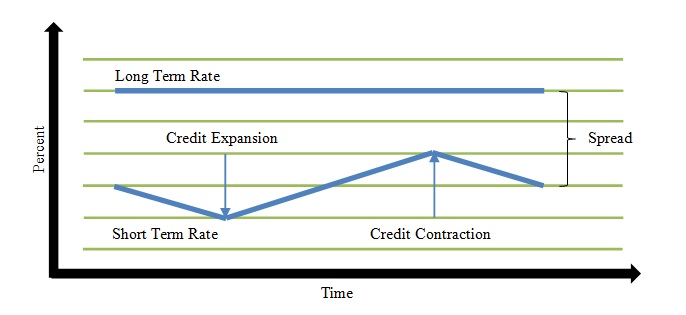
A graphical representation of the Austrian Cycle Theory is presented in Figure 2.
Figure 2: The Austrian Business Cycle Theory (Created by author based on the data acquired from Huerto de Soto, J., 2013).
If borrowers perceive that the greater amount of available funds is a result of an increase of available funds in the investment and consumer spheres, the investors would not have been aware of the impending restriction in funds. This misperception is a result of the investor’s lack of awareness that the positive investment environment was a result of a manipulation in monetary policy and not as result of organic economic growth. Understanding the impact of interest rates on investments is critical to understanding true demand, as opposed to artificially-induced demand. While there are many variables involved in the process, one can at least expect the prices of commodities and high-order capital goods to decline after the central bank announces an increase in the rate.
To conclude the section on the Austrian Business Cycle Theory, it is worth to summarize the main points: this theory suggests that government manipulations in the credit market inevitably result in asset bubbles, unsustainable business expansion and, ultimately, recession. Unlike other macroeconomic explanations of the business cycle, the Austrian theory argues that government attempts to stimulate economies and shorten recessions are ineffective and counterproductive. The theory assumes that interest rate is used to coordinate spending, saving, lending and investment. Large, long-term manipulations of the interest rate lead to too much investment in the wrong industries, creating the illusion of real economic growth. The factors of production and business capital flow into wasteful, unsustainable endeavors. All these mistakes become unprofitable and lead to a recession. The labor and investment that was employed towards inappropriate industries (such as construction and remodeling in 2008) need to be redeployed towards actually economically feasible ends. This short-term business adjustment causes real investment to drop and unemployment to rise. The government or central bank might attempt to circumvent the recession by lowering interest rates or propping up failed industry. Austrian theorists believe that this would only cause further malinvestment and make the recession that much worse when it actually strikes (Investopedia, 2017b).
The Kondratieff Long Economic Cycles
The second cycle of interest is the Kondratieff cycle (also called Kondratieff (also spelled Kondratiev) waves, long waves, long economic cycles, K-waves) (Grinin L., Korotayev A., and Tausch A., 2016). The theory was developed by Russian scientist & economist Nikolay Kondratieff (1892 – 1938) who is credited with launching the idea of long economic cycles (Grinin L., Korotayev A., and Tausch A., 2016). The theory hypothesized the existence of very long-run macroeconomic and price cycles, originally estimated to last 50-54 years. Kondratieff viewed depressions as cleansing periods that allowed the economy to readjust from the previous excesses and begin a base for future growth. The characteristic of fulfilling the expectations of the previous period of growth is realized within the secondary depression or down grade. This is a period of incremental innovation where technologies of the past period of growth are refined, made cheaper, and more widely distributed. Within the downgrade is a consolidation of social values or goals. Ideas and concepts introduced in the preceding period of growth, while sounding radical at the time, become integrated into the fabric of society. These social changes are often supported by shifts in technology. The period of incremental innovation provides the framework for social integration.
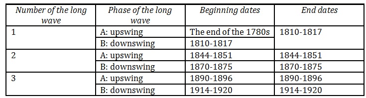
His ideas gained more prominence posthumously after Schumpeter published his distinguished work on the business cycle and named the long cycles Kondratieff cycles in his honor (Rumyantseva S., 2003). The theory itself denotes that there are long-term cycles of about 50 years in length that are made up: “[…] of phases of gradual increases in value of respective indicators followed by phases of decline” (Korotayev, A., and Tsirel, S., 2010). Kondratieff identified several types of these cycles in history and their respective phases. The long waves and their phases identified by Kondratieff are presented in Table 1.
Table 1: Long Waves and their Phases identified by Kondratieff (Created by author based on the data acquired from Korotayev, A., and Tsirel, S., 2010)
Several explanations developed over time in regard to the underlying causes for the observed cycles. Kondratieff accounted for the existence of these cycles on the basis of capital investment dynamics (Kondratieff, N., 1928; Kondratieff, N., 1984). Kondratieff’s analysis described how international capitalism had gone through many “great depressions” as these were a natural part of the international mercantile credit system. The long-term business cycles that he identified through meticulous research are now also called “K” waves. The K wave is a 60 year cycle (+/- a year or so) with internal phases that are sometimes characterized as seasons: spring, summer, autumn and winter:
Spring phase: a new factor of production, good economic times, rising inflation;
Summer: hubristic ‘peak’ war followed by societal doubts and double-digit inflation;
Autumn: the financial fix of inflation leads to a credit boom which creates a false plateau of prosperity that ends in a speculative bubble;
Winter: excessive capacity worked off by massive debt repudiation, commodity deflation & economic depression (Quigley, C., 2012).
Later researchers postulate that the cycles are connected with new phases of technological innovation (Grinin L., Korotayev A., and Tausch, A., 2016; Korotayev, A., and Tsirel, S., 2010). Where one could apply this knowledge, however, is in forecasting long-term movements in the economy related to technological innovation. Over last two centuries, different innovations have triggered the phase of growth. The first peak was for the textile industry in 1815, the second one for the railway steel with a peak was in 1873, and then a new cycle was caused by electro-technology, before decreasing since 1920. Then we could observe the automobile revolution, so the economy grew up until 1973, finally we can observe the information-technology innovation for 1990 with a peak in 2002. For example, the Internet revolutionized the scope of markets and led to a period of rapid economic growth during the 1990’s and 2000’s. Today, one can argue that the global economy has adjusted to this development. Opportunities for start-ups to expand are not as plentiful as is reflected on a macro-level with chronic low GDP growth across the developed world. One may apply Kondratieff cycle theory to explain the low GDP growth as well. For the future, we can imagine innovations in health sector at the origin of a new cycle.
To conclude this section, we should note that Kondratieff long-term cycle theory describes the features of the economic activity of capitalist nations, and that they involve periods of evolution and self-correction. The K-Wave cycle theory was watched closely 50 years following the market crash of 1929, after which it was deemed pertinent to economic and political cycles (Investopedia, 2017a).
The Elliott Wave Theory
The Elliott Wave is a theory established by Ralph Nelson Elliott (1871 – 1948), an American financial accountant, in the 1930s. It is a form of technical analysis which can be used to analyze financial market cycles and forecast market trends (Atsalakis, G., Dimitrakakis, E., and Zopounidis, C., 2011; Chen L., Cheng C., and Teoh H., 2007; Frost, A., and Prechter, R., 2005). Elliott postulated that stock markets do not behave randomly, instead claiming that they move in repeating cycles which reflect the emotions and actions of humans that are the results of mass psychology (Chen L., Cheng C., and Teoh H., 2007). These patterns that Elliott coined “waves” are “[…] repetitive in form but not necessarily in time or amplitude” (Kotick, J., 1996). These waves connect with each other to establish bigger versions of the pattern with this cycle repeating itself.
Ralph Nelson Elliott developed the Elliott Wave Theory by discovering that stock markets which are thought to behave in a somewhat chaotic manner, in fact traded in repetitive cycles. Elliott discovered that these market cycles resulted from investors’ reactions to outside influences, or predominant psychology of the masses at the time. He found that the upward and downward swings of the mass psychology always showed up in the same repetitive patterns which were then divided further into patterns; he termed “waves”.
Elliott’s theory is based on the Dow theory in that stock prices move in waves. Because of the “fractal” nature of markets, however, Elliott was able to break down and analyze them in much greater details. Fractals are mathematical structures, which on an ever-smaller scale, infinitely repeat themselves. Elliott discovered that stock-trading patterns were structured in the same way.
Elliott made detailed stock market predictions based on unique characteristics that he discovered in the wave patterns. An impulsive wave which goes with the main trend always shows five waves in its pattern. On a smaller scale, within each of the impulsive waves, five waves can again be found. In this smaller pattern, the same pattern repeats itself ad infinitum. These ever-smaller patterns are labeled as different wave degrees in the Elliott Wave Principle. Only much later were fractals recognized by scientists. We know that in international financial markets “every action creates an equal and opposite reaction” as a price movement up or down must be followed by a contrary movement. Price action is divided into trends and corrections or sideways movements. Trends show the main direction of prices while corrections move against the trend. Elliott labeled these; “impulsive” and “corrective” waves.
To conclude this section, it is important to mention that Elliott Wave Theory has its devotees and its detractors like many of the other technical analysis theories out there. After analyzing the patterns of the Elliott Wave, it is clear, through technical analysis, that there is a fairly predictable pattern in this theory. The difficult part deciphering which part of the Elliott Wave one is experiencing. One of the key weaknesses is that the practitioners can always blame their reading of the charts rather than the weaknesses in the theory or vice versa. Failing in that, there is the open-ended interpretation of how long a cycle takes to complete (Investopedia Staff, 2017).
The Juglar Cycle Theory
The Juglar Cycle is an economic cycle that lasts between 7-11 years and is therefore deemed a medium-term cycle (Schumpeter, J., 1950). The Juglar Cycle also appears under the name “business cycle” (Grinin L., Korotayev A., and Tausch, A., 2016). In 1862, Clement Juglar became one of the first to discover and describe the cycle (Grinin, L., Korotayev, A., and Malkov, S., 2010; Grinin L., Korotayev A., and Tausch, A., 2016; Juglar, C., 1862; Juglar, C., 1916; Morgan, M., 1990). Juglar believed that a financial crisis accompanied by panic is not an isolated phenomenon but one of the three stages of social economic development; which are prosperity, crisis and depression. The recurring of the three stages leads to the fixed cycle. Juglar also demonstrates that the crisis is a normal social phenomenon in developed business and industries which can be foreseen and eased by some kind of measures but impossible to be totally inhibited. It is not politics, war, failed harvesting and climate change that are the reasons of the cycle (Juglar, C., 1916). Juglar cycle is a phenomenon that occurs automatically which has a direct relationship to people’s behavior, saving habits and how citizens use their capital. British economist Hanson calculated that an average Juglar cycle is 8.35 years, based on the British statistics from 1795 to 1937.
Whereas the Kondriateff cycle had technological phases of innovation as its catalyst, the Juglar cycle is driven by both “[…] investment and innovation aspects […].” (Rumyantseva, S., 2003). The cycle consists of several fluctuations between economic growth, boom, and finally downturn, after which a new cycle is started. As stated by Grinin et al. in their 2016 book:
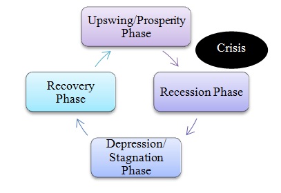
“[The Juglar Cycle] can be subdivided into four phases: (1) phase of recovery, when, after the fall of production and stagnation, economic growth begins; (2) expansion phase, when economic growth is accelerating up to an economic boom; (3) phase of recession, during which the euphoria of prosperity is replaced by panic accompanying collapse, and after that comes the economic down- turn; (4) phase of depression or stagnation, during which a balance is achieved: the decline has stopped, but any pronounced growth is absent yet” (Grinin L., Korotayev A., and Tausch, A., 2016).
Figure 3 illustrates the nature of the cycle and its four phases.
Figure 3: The model of a Juglar Cycle (Created by author based on the data acquired from Grinin L., Korotayev A., and Tausch, A., 2016)
The Juglar Cycle is particularly useful in understanding the general behavior of recessions. The Dot-Com bubble crash occurred in 2001, just seven years before the Great Recession of 2008. These two recessions fit into the Juglar Cycle theory and could potentially be useful to investors. The market is only 9 years removed from the beginning of the last recession. The cycle is 7 to 11 years length and the reasons for it lies in how Americans use their money and capital. For example, after the Second World War was over, the US government consumed substantial amounts of money and capital to rebuild the public system which was damaged during the war, which automatically lead to another prosperity part of the new cycle.
By virtue of the Juglar Cycle, one can deduce that the economy is “due” for a contraction during the next three years. A savvy investor could accrue capital during this time. Once the recession strikes, the investor could invest heavily into major indices with reasonable theoretical assurances that the market should trend upward over the following 7 to 11 years.
The existence of the Juglar cycle, and cycles in general, is still denied by economists such as Gregory Mankiw (Mankiw, N., 2014) which warrants a closer examination of the empirical evidence of Juglar cycles. Korotayev and Tsirel investigated the existence of several types of cycles, such as the aforementioned Kondratieff cycle and the Juglar cycle, with the help of a spectral analysis. They concluded that “[…] the reduced spectra analysis has indicated a rather high (2–3%) significance of Juglar cycles (with a period of 7–9 years), as well as the one of Kitchin cycles (with a period of 3–4 years). Thus our spectral analysis has also supported the hypothesis of the presence of Juglar and Kitchin in the world GDP dynamics”(Korotayev, A., and Tsirel, S., 2010).
Short Term Cycle Theories
While the business cycle is a relatively simple concept, there is a great debate among economists as to what influences the length and magnitude of the individual parts of the cycle (Simpson, S., 2017). Let us now turn to the short-term cycles and investigate several selected short-term cycle theories such as: the Kitchin Сycles, the Presidential Election Cycles, and the Lehman Wave Theory.
The Kitchin Cycle Theory
The Kitchin Cycle is important to understanding inventory management and the flow of the supply chain. Kitchin cycles are short-term cycles with a length of 3-5 years which reflect fluctuations in inventory levels (Brouwer, M., 2016). They were identified by and named after British economist and statistician Joseph Kitchin who published his findings in 1923 in his text Cycles and Trends in Economic Factors. Rumyantseva offers a clear synopsis of the cycle:
“The logic of this cycle can be described in a rather neat way through neoclassical laws of market equilibrium and is accounted for by time lags in information movements affecting the decision making of commercial firms. As is well known, in particular, firms react to the improvement of commercial situation through the increase in output through the full employment of the extent fixed capital assets. As a result, within a certain period of time (ranging between a few months and two years) the market gets ‘flooded’ with commodities whose quantity becomes gradually excessive. The demand declines, prices drop, the produced commodities get accumulated in inventories, which informs entrepreneurs of the necessity to reduce output. However, this process takes some time” (Rumyantseva, S., 2003).
The lag in time between recognizing that the output is too high and reducing the output generates the Kitchen cycles (Van Duijn, J., 1977). However, reducing the output sets the stage for a new phase of demand growth which restarts the cycle (Kitchin, J., 1923).
According to David Glasner in his book Business Cycles and Depressions (Glasner D., 1997); if the existence of major cycles of 7 to 10 years had been already well established, the 40 months cycles however were a new observation. Kitchin assumed that major cycles were simply composed of two to three minor cycles. After observing monthly statistics on bank clearings, commodity prices, and short-term interest rates in the United-States and Great Britain from 1890 to 1922, he concluded that all three series were apparently moving together in roughly 40 months’ cycles. The range of proposed factors causing business cycles is wide: from climate, overinvestment, monetary, underconsumption to psychological factors. Kitchin explained the cyclical movements in economic activity by the fact that the capitalist process reflects rhythmical movements in mass psychology. But they can also be explained by the fact that through prices of basic food, cyclical movements can be influenced by the excess or insufficiency of crops which might fall out of step with the normal cycle. Food prices are however influenced by crops on one hand and by cyclical fluctuations on the other hand. The approximate recurrence of cycles, however, suggests more the inconstant recurrence of human behavior. Therefore, according to Joseph Kitchin, the cycles were not exact because of the nature of human behavior and because factors like food production might fall out of step with the normal cycle.
The 40-month Kitchin Cycle is signaling slower business formation, extremely weak consumer demand, slower inventory turnover and chronic unemployment. The cycle is believed to be accounted for by time lags in information movements affecting the decision making of commercial firms. Firms react to the improvement of commercial situation through the increase in output through the full employment of the extent fixed capital assets. As a result, as was already described at the beginning of this section within a certain period of time (ranging between a few months and two years), the market gets ‘flooded’ with commodities whose quantity becomes gradually excessive. The demand declines, prices drop, the produced commodities get accumulated in inventories which informs entrepreneurs of the necessity to reduce output (Wikipedia, 2017; Time-Price-Research, 2015).
To conclude this section, it is worth noting that Kitchin offered little theoretical explanation for the cyclical movements in economic activity. He thought that the capitalist process merely reflected rhythmical movements in mass psychology. The cycles were less than exact because of the nature of human behavior, and because factors like food production might fall out of step with the normal cycle.
The Presidential Election Cycle Theory
The presidential election cycle theory was first developed by stock market historian Yale Hirsch. Hirsch’s theory postulates that there is a correlation between stock market performance and the presidential election cycle (Sturm, R., 2009; Thune, K., 2016). According to the theory, every year in the presidential cycle exhibits a particular performance trend in the stock market depending on the political climate and measures of the president in office and is restarted again after re-election (Lewis, N., 2016). The presidential election cycle theory has been the topic of numerous publications over the years (Allivine, F., and O’Neil, D., 1980; Gärtner, M., and Wellershoff, K., 1995; Hirsch, Y., 2015; Huang, R., 1985; Johnson, R., Chittenden, W., and Jensen, G., 1999; Nordhaus, W., 1975; Sturm, R., 2009; Umstead, D., 1977; Wong, W.-K., and McAleer, M., 2009), references to which provide relevant information.
The presidential cycle theory suggests that there is a link between the US four-year presidential term and the US stock market prices (Ficenec, J., 2014). Contemplating on this, Yale Hirsh (Hirsch, Y., 2004) theorized that the presidential elections that happen every four years have a significant impact on the US economy and stock market. Moreover, Hirsch postulated that “wars, recessions and bear markets tend to start or occur in the first half of the term and bull markets, in the latter half.” In general, it is proposed that the US stock prices have a weaker performance during the first two years of presidency and consequently perform stronger during the second half of the presidency (Wong, W.-K., and McAleer, M., 2009). In this case, the stock performances somewhat usually bottomed in the second year and rose the most during the third year of the presidential election cycle (Beyer, S., Jensen, G. and Johnson, R., 2008). It is theorized that the main reason for this correlation comes from the notion that ahead of elections politicians try to promote a pro-business agenda in the general economy, so that the “economy is strong, stock market is bullish, and voters are upbeat heading to the polls” (Lee, P., 2013). So, in essence, what usually is predicted to happen is that the government in power tries to adjust the prevailing macro and microeconomic policies to achieve re-election or some other kinds of political agendas (Wong, W.-K., and McAleer, M., 2009).
After a new president has been elected, the public is often in a kind of “honeymoon period” when they feel a high from the election circus and are looking forward to the new president. The presidential cycle theory suggests that around this time, the governmental decision makers begin to feel less pressured about the policies or initiatives they are dealing with, and so they start introducing more restrictive and unpopular policies than when they were closely under scrutiny. Often, these new initiatives involve the raising of taxes, higher spending and more legal regulation which all together serve to impact consumers and businesses negatively. Eventually, these measures get reflected in the stock market and a negative feedback loop commences. The bottoming of the situation then usually takes place during the second year of the cycle when the US Presidential term and the Mid-term elections cross paths. Around this time, the party in power performs relatively poorly at the polls, ultimately, resulting in the politicians in power changing their policies in to a more positive direction looking at the Presidential elections soon ahead (Lee, P., 2013).
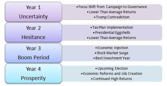
Let us make an analysis of the stock market performance based on each US presidency term year. As we have already described, the first half of a president’s term is characterized by weaker or below average returns in the stock market, whereas the second half consists of bull markets and above-average returns (Hirsch, Y., 2015). The theory goes even further, providing a prediction of the stock market returns for every year of the presidential term. The first year after election is the weakest of the four because the president is still acclimating to his new position (Frownfelter, J., 2016) and trying to honor campaign promises, which often involve less popular acts such as increasing tax rates, government regulations, and spending (Borzykowski, B., 2016; Hawkins, J., 2011). The second year typically sees higher returns than the first in terms of stock market performance but still falls in the below average spectrum (Frownfelter, J., 2016) because, according to its inventor Hirsch: “Wars, recessions, and bear markets tend to start or occur in the first half of the term[…]” (Hirsch, Y., 2015). The third year marks the start of the second half of the president’s term in office and the beginning of the prosperous period (Hawkins, J., 2011). As Sturm puts it, this is due to:
“The basic argument is that politically motivated fiscal, economic and administrative policies can inject additional cash flow into the economy and the stock market in the second half of presidential administrations to enhance the re-election chances of the candidate of the party holding the presidency” (Sturm, R., 2009).
On average, the third year of the presidency correlates with the highest stock market returns because the president’s administration attempts to produce a robust economy in an effort to increase chances of re-election. The fourth year offers lower returns but still above those of the first half (Hawkins, J., 2011; CTS Financial Group, 2016). Figure 4 provides a brief summary of the observations.
Fig. 4: Yearly Breakdown of the Presidential Election Cycle (Created by author)
Nordhaus analyzed a total of nine countries and concluded that only three of these (Germany, New Zealand and the United States) exhibited a correlation between business cycles and political cycles based on unemployment rates between 1947 and 1972 (Nordhaus, W., 1975). In their landmark study, Allvine & O’Neill asserted that apart from the short run, “[…] changes in stock prices are essentially not random.” They investigated S&P 400 data for the period of 1948-1978 in relation to presidential terms and concluded that: “[…] The results indicate a clear relation between stock returns and the presidential cycle” (Allivine, F., and O’Neil, D., 1980).
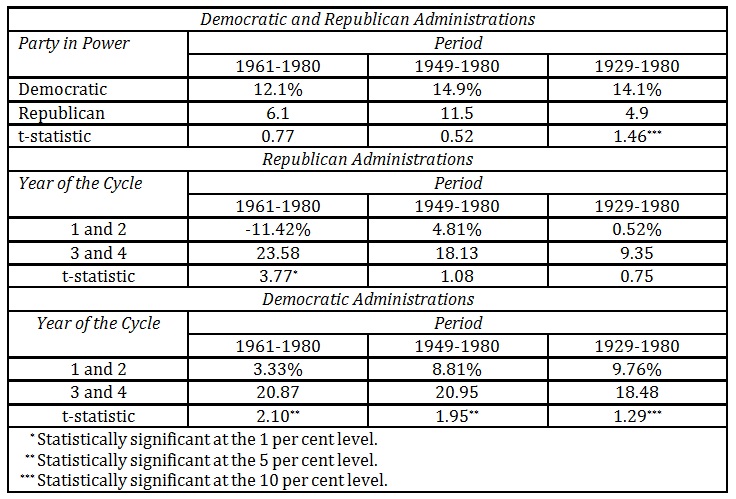
In 1985, Huang followed a similar approach to Allvine & O’Neill with somewhat mixed results. Huang wrote: “The results of formal statistical tests are somewhat mixed. Nonetheless, the pattern is hard to ignore” (Huang, R., 1985). He extended the research by analyzing whether the cycle favors one of the two major parties, namely, Republicans or Democrats. As can be seen in Table 2, Democratic administrations experienced greater stock market returns than Republican administrations.
Table 2: Mean annual returns depending on administration (Created by author based on the data acquired from Huang, R., 1985).
The next article to investigate the presidential election cycle theory appears in 1995, more than ten years after Huang’s investigation. Gärtner and Wellershoff looked at different stock indices such as the S&P 500, the NASDAQ composite index, and the Dow Jones Industrial Average during the period from 1961 to 1992. They conclude that the presidential election cycle theory is statistically significant across all indices and varying administrations. However, they disagree with Huang’s assessment that democratic administrations enjoy greater stock market returns (Gärtner, M., and Wellershoff, K., 1995). Gärtner and Wellershoff’s sentiment is shared in several other articles (Johnson, R., Chittenden, W., and Jensen, G., 1999; Siegel, J., 2008; Smith, K., 1992). The general consensus was that there is no significant difference in stock market returns between Democratic and Republican administrations. In their 1999 paper, Johnson, Chittenden, and Jensen analyzed the stock market performance between 1929 and 1996 and stated that: “Our findings generally support prior research that shows stock returns are significantly higher in the second half of the term” (Johnson, R., Chittenden, W., and Jensen, G., 1999). Interestingly, the same did not hold true for bond returns between the first and second half of a presidential term.
In 2009, Wong and McAleer tested the presidential election cycle theory once again, reaching the conclusion that: “[…] there were statistically significant Presidential Election Cycles in the US stock market during the greater part of the past four decades, at both the overall as well as individual levels” (Wong, W.-K., and McAleer, M., 2009).
The final empirical investigation that we want to emphasize was conducted by the same man who is credited with discovering the presidential election cycle theory. Hirsch analyzed stock market returns from the period of 1833 to 2013 (181 years) based on the annual % change in the Dow Jones Industrial Average.
Hirsch reached the conclusion that his theory is valid as the post-election year experienced the lowest growth out of all four years, with the mid-term year doing marginally better. Taken across this 181-year period, the pre-election year experienced the biggest stock market gains while the election year was worse off but still well above both years of the first half of the term (Hirsch, Y., 2015).
In conclusion, we would like to finalize several observations. First, investors should keep in mind that the theory postulates a correlation between the presidential cycle and the stock market returns and not a causal relationship. Second, the methodology across the aforementioned academic journals differ significantly in both time periods sampled, the underlying data analyzed, the scope of analysis (individual years, two halves of the term, entire terms, aggregates) and statistical methods (t-tests, spectrum analysis). By aggregating individual terms into larger groups of data and merely looking at the averages, individual years which refute the cycle are ignored. Third, the underlying causes have not been thoroughly analyzed or, in regard to the original reasons put forth by Nordhaus, refuted (McCallum, B., 1978). Fourth, the past does not necessarily predict the future as one may simply mistake noise in the data for the signal or engage in the cognitive deception of wanting to see patterns (Silver, N., 2012). Further research is necessary in order to establish the fundamental mechanics at work behind the presidential election cycle theory. However, this does not render the theory useless. There is an evidence (Hirsch, Y., 2015) that there is at least a correlational relationship between the Presidential Pre-Election Year and larger than average returns. One could take advantage of post-election uncertainty and invest during the first year of the cycle. Looking at one’s investments with a three to four-year horizon should provide opportunities to grow one’s wealth by divesting before uncertainty begins to grow again during the following election year, the fourth year of the cycle.
The Lehman Wave Theory
The Lehman Wave is the name given to the synchronized bullwhip-like effect that simultaneously hit all markets following the bankruptcy of Lehman Brothers in September 2008 (Peels, R., Udenio, M., Fransoo, J., Wolfs, M., Hendrikx, T., NeoResins, D., and Fransoo, J., 2009). The observed effect persisted between 12 and 16 months. Peels et al. argue that Lehman Brothers’ bankruptcy caused a global de-stocking effect to reduce operating working capital and increase cash reserves. The de-stocking effect led to a decrease in sales and, similar to the bullwhip effect (Lee H., Padmanabhan V., and Whang, S., 1997), the drop in sales was greater for companies situated further upstream in the supply chain (Peels, R., Udenio, M., Fransoo, J., Wolfs, M., Hendrikx, T., NeoResins, D., and Fransoo, J., 2009). The same researchers developed a model to predict when the shock created by Lehman wave would subside and demand would return to normal economic levels (Steen, M., 2009). As stated in an article in the Financial Times, the researchers “[…] believe the model is especially helpful in guiding companies at the ends of long supply chains who may overreact in a crisis by closing down plants too quickly and then discover they cannot deal with demand in the recovery” (Steen, M., 2009).
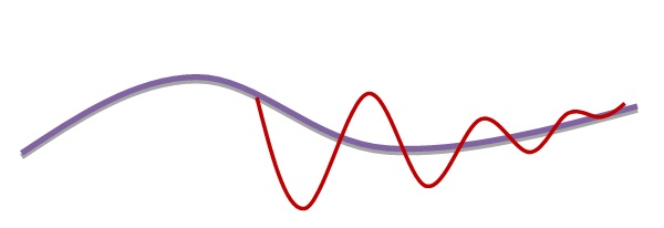
Figure 5 offers a visualization of the Lehman wave.
Figure 5: The Lehman Wave (Created by author based on the data acquired from Peels, R., Udenio, M., Fransoo, J., Wolfs, M., Hendrikx, T., and De Vreeze, D., 2010).
Lehman wave (red on Fig. 5) with a wavelength between 12 and 16 months on top of the longer term economic wave (blue on Fig. 5), with a wavelength of 5 to 10 years. Peels et al. offer the following explanation for its wave character:
“It is a wave because the value chain system is elastic: all companies constantly strive to keep their optimal equilibrium, but due to delay factors are always overshooting. The Lehman wave is dampened, because all companies take time to respond to changes in demand. Like any other wave, the Lehman wave has a wavelength, which is determined by the medium in which it oscillates, thus by the parameters of the supply chain. The amplitude of the Lehman wave is determined by the force of the pulse that caused it” (Peels, R., Udenio, M., Fransoo, J. C., and Griffioen, S., 2011).
To avoid taking costly loans and assure the company’s liquidity, enterprises rather concentrated on reducing costs in every possible field. Many of them focused on de-stocking, but also cutting down working capital e.g. in inventories. As a matter of fact, it complicated the daily business regarding traditional forecasting. Normally, a combination out of the three following operations would have been used: customer information; but customers did not know what to expect; historical data; failed to reach any solution, and finally the third one is current sales; which dropped sharply. Consequently, the process of forecasting became unreliable. To understand the mechanism of the Lehman Wave better, it is necessary to give a few explanations concerning the appearing flows of downward and upward streams in the supply chain management.
The distinction of the flows in upward and downward streams in the supply chain model is as following: the upward stream in the production process can be seen as information and extracting flow concerning the orders of customers and raw materials; which goes upstream. Meanwhile the downward stream represents the material flow concerning the deliveries and the actual sale of the finished product to customers or other businesses, and goes downstream (Bass, B., 2017). Furthermore, it is important to understand two different terms of de-stocking in the context of supply chain to model the different phases of the process-oriented process probably. First of all, active-destocking needs to be taken into consideration: the reduction of the actual necessary inventory level is required to enhance efficiency and to save money due to a deliberate management decision. The supply chains expand during crisis, in case of a conscious and active reduction of multiple downstream enterprises of the demanded inventory coverage. This can be seen as a vicious circle, because it takes the form of a cumulative effect in the chain. Consequently, if there is the existence of various layers in the supply chain, it can cause financial loss of sales upstream up to 60 days (Stein W., 2010). The second term is re-active de-stocking and is the process to reduce stock level in case of decreasing sales. When the demand declines, there is less desired inventory coverage necessary; consequently, the forecast and the actual stock purchases will also decline. This reaction is slowed down; therefore, the effect also comes delayed.
The Lehman Wave is driven by significant disruptions of the economic system that occur suddenly. The mechanism is a weakened wave-like variation around a harmonized balance. The reason for defining end-markets is the following: the previous mentioned researchers also found out that the complexity and the range of the Lehman-Wave is smaller for businesses that are closer to its end markets due to the gap caused by cumulative reduction of inventory of the supply chain, than business which are more distanced to its end markets.
To summarize, the Lehman Wave can have significant impacts on the sales volume. This, in turn, significantly influences the profitability of those enterprises which mainly rely on an upstream flow in their supply chain. The mentioned bankruptcy of the Lehman Brothers caused a sudden summit in the interest rate of London Interbank Offered Rate (LIBOR) used as the worldwide benchmark for short-term interest rates which resulted in bank’s revocation of credit and redundancy of cash by decreasing stocks. End markets in many markets responded with various strength of decline concerning the economic wave, but the main driver was the de-stocking which implied weakened wave-like effects, namely; the Lehman Wave. When a recession occurs, investors are prone to panic and are often quick to pull their capital out of the markets. The Lehman Wave shows that such a market exodus only exacerbates the problem.
Problem Statement
Based on the conducted analysis of long and short-term cycle theories, the goal is to choose the most suitable wave theory and apply it to determine the stocks with the highest investment attractiveness and growth potential from three asset classes:
1) Hospitality Real Estate Investment Trusts (HREITs);
2) International Hospitality Groups (IHGs) or International Groups with significant investment in the hospitality sector;
3) International Hotel Chains (IHCs).
In the next section, relevant investigation will be conducted and the outcomes will be presented. The most promising investments from each determined asset class will be selected and the choice would be justified.
Investigation framework and proposed solutions
First, the most relevant cycle theory will be selected based on the stated problem. The investigation timeframe encompasses a 5-year time horizon: from January 2010 to January 2015. The stock price performance of each investment is examined over this timeframe.
Investigation is performed for the following investment classes:
1) Hospitality Real Estate Investment Trusts: Chatham LT; Chesapeake LT; RLJ Lodging Trust; Pebblebrook HotelTrust; Hospitality PT.
2) International Hospitality Groups: Shanghai Jin Jiang HG; HomeInns Group; NH Hotel Group; Blackstone Group; Inter Continental HG.
3) International Hotel Chains: Accor Hotels; Choice Hotels; Hyatt; Starwood, Wyndham Worldwide.
Based on the conducted analysis, the Elliott Wave Cycle Theory application was chosen for the stated problem. Based on the extensive analysis of the Elliott Wave Theory, we came to the conclusion that it provides more gain for the risk given the stated problem we are to solve in this article. Furthermore, based on our investigation, the argument that market cycles could be traced back to outside influences put forth in the Elliott Wave Theory along with the predominant psychology of market participants would allow us to get the most accurate results for assessing the market attractiveness and growth potential of the hospitality market investment classes over the 5-year period. According to our analysis, the shifts in mass psychology which result in repetitive patterns are best mathematically categorized into the impulsive and corrective waves by the Elliott Wave Theory. Hence, the Elliott Wave Theory allows making detailed stock market predictions based on unique characteristics in the wave patterns. After analyzing the patterns using this particular wave theory, given that the investigation timeframe is long enough (5 years), it is possible to forecast the potential stock price growth with a high degree of certainty.
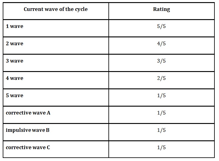
Table 3 presents the assessment framework for the stock price trends within the framework of the wave theory (Kostin, K., 2016).
Table 3: The assessment framework (Created by author based on the analysis of the Elliott Wave Theory)
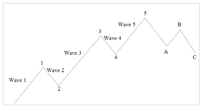
The mechanism of assessment interpretation presented in table three could be formulated as follows. An impulsive wave, which goes with the main trend, always shows five waves in its pattern. On a smaller scale, within each of the impulsive waves, five waves can again be found. In this smaller pattern, the same pattern repeats itself ad infinitum. Price action is divided into trends and corrections or sideways movements. Trends show the main direction of prices while corrections move against the trend: “impulsive” and “corrective” waves. Waves 1, 3, and 5 are the “impulsive waves”, and waves 2 and 4 – the “corrective waves”. The stock price increases with each “impulsive wave” and decrease with each “corrective wave”, however in such a pattern that for each new wave the peak is higher than the previous peak (please refer to Figure 6).
Fig. 6: The cycle model within the framework of the Elliott Wave Theory (Created by author based on the analysis of the Elliott Wave Theory).
The maximum at the end of the 5th wave is considered the peak price indicator for the cycle. At the end of the 5th wave, the corrective phase begins. The correction disintegrates into three subsequent waves: two corrective waves (A and C) and one impulse wave (B). After that, the new cycle begins. Hence, we observe four impulsive waves and four corrective waves in one cycle.
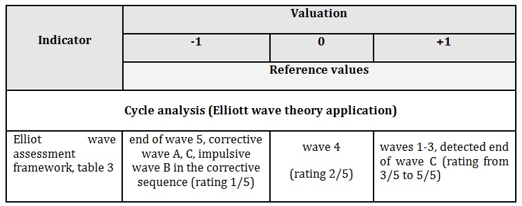
The overall investment attractiveness evaluation is performed in accordance with the framework presented in table 4.
Table 4: Comprehensive criteria for investment attractiveness evaluation (Created by author)
Results
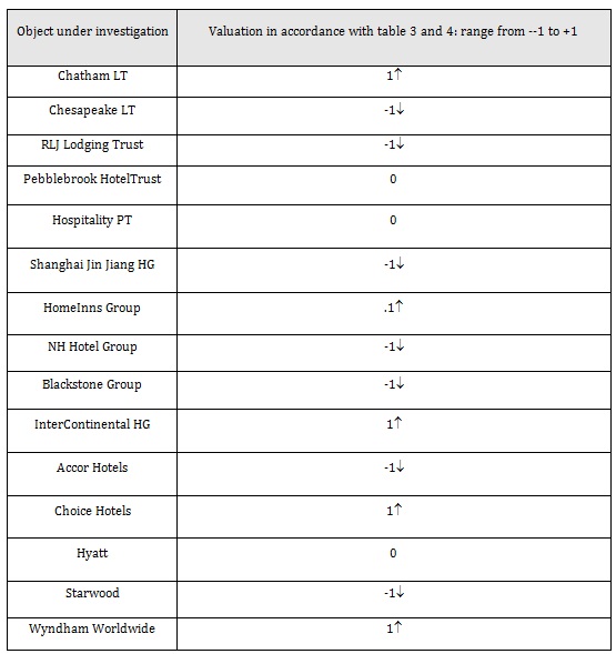
After the application of the proposed assessment framework, the following results presented in table 5 were obtained for the three investment classes under investigation: 1) Hospitality Real Estate Investment Trusts; 2) International Hospitality Groups or International Groups with significant investment in the hospitality sector; and 3) International Hotel Chains.
Table 5 : The results of investment attractiveness assessment of the global companies (Created by author).
The practical application of the proposed investment attractiveness evaluation based on the selected Elliott Wave Cycle Theory was demonstrated. Within the framework of the proposed method, the investment attractiveness of 15 global companies representing the tourism and hospitality industry was evaluated. The following most prosperous investment opportunities were determined:
1) Among the HREITs, Chatham LT is suggested as the most promising investment opportunity;
2) Among the IHGs or IG, HomeInns Group and Intercontinental HG are suggested as the most promising investment opportunities;
3) Among the IHCs, Choice Hotels and Wyndham Worldwide are suggested as the most promising investment opportunities.
Conclusions
Based on the analysis conducted, it could be concluded that different cycle theories help understand, explain and predict the measures the governments are likely to take and determine among others such important economic factors as the interest rates, inflation rate and the general state of the economy. For example, interest rates usually follow the trends shaped by the economic cycles. During the recession interest rates are likely to slow down along with the economy and during the expansion interest rates increase. When interest rates increase, the value of the currency increases, driving up the value of the currency. The opposite holds true as well. Based on the interest rates’ trends, which could be identified via the economic cycle analysis, investors could craft relevant investment strategies when investing in various currencies. Economic cycle theories could be regarded as tools to analyze the economy and forecast the potential state of the economy. The general state of the economy and the rate of inflation are very much related to the notion of the economic cycle, as both indicators follow the cycle trends. In point of expansion, economy is growing and inflation rates are increasing as well. During the recession, both are slowing down. By following the inflation rate, investors and global companies can estimate and forecast other countries’ economic state. Based on the economic cycle, they are also able to evaluate profitability of their investments. Hence, profitability of certain investments and failure of others could be forecasted.
Economic cycles can be defined as fluctuations in the aggregate economic activity of a country which take place on a repeating basis over a number of months or years. Market economies are characterized by two main periods, a long-term growth trend and more or less significant short-term fluctuations in activity around this trend. The Austrian Business Cycle Theory suggests that government manipulations in the credit market inevitably result in asset bubbles, unsustainable business expansion and, ultimately, recession. The theory assumes that interest rate is used to coordinate spending, saving, lending and investment. Large, long-term manipulations of the interest rate lead to too much investment in the wrong industries, creating the illusion of real economic growth. The factors of production and business capital flow into wasteful, unsustainable endeavors. The Kondratieff theory hypothesized the existence of very long-run macroeconomic and price cycles, originally estimated to last 50-54 years. Kondratieff viewed depressions as cleansing periods that allowed the economy to readjust from the previous excesses and begin a base for future growth. The characteristic of fulfilling the expectations of the previous period of growth is realized within the secondary depression or downgrade. This is a period of incremental innovation where technologies of the past period of growth are refined, made cheaper, and more widely distributed. Within the downgrade is a consolidation of social values or goals. Ideas and concepts introduced in the preceding period of growth, while radical sounding at the time, become integrated into the fabric of society. These social changes are often supported by shifts in technology. The period of incremental innovation provides the framework for social integration. The Elliott Wave Theory is a form of technical analysis which can be used to analyze financial market cycles and forecast market trends. Elliott postulated that stock markets do not behave randomly, instead claiming that they move in repeating cycles which reflect the emotions and actions of humans that are the results of mass psychology. The Juglar Cycle is an economic cycle that lasts between 7-11 years and is, therefore, deemed a medium-term cycle. Juglar believed that a financial crisis accompanied by panic is not an isolated phenomenon but one of the three stages of social economic development which are prosperity, crisis and depression. The recurring of the three stages leads to the fixed cycle. The Kitchin Cycle is important to understand inventory management and the flow of the supply chain. Kitchin cycles are short-term cycles with a length of 3-5 years which reflect fluctuations in inventory levels. The Presidential Election Cycle Theory was first developed by stock market historian Yale Hirsch. Hirsch’s theory postulates that there is a correlation between stock market performance and the presidential election cycle. According to the theory, every year the presidential cycle exhibits a particular performance trend in the stock market depending on the political climate and measures of the president in office and is restarted again after re-election. The Lehman Wave Theory is the name given to the synchronized bullwhip-like effect that simultaneously hit all markets following the bankruptcy of Lehman Brothers in September 2008. The observed effect persisted between 12 and 16 months.
Based on the fluctuation of economic cycle investors and companies who are thinking about starting a new business in another country, investing foreign currency or investing assets in other country have to take into consideration the economic cycles of that country that they are planning to invest in. By understanding the phases of the economic cycles, business entities and investors could also infer the future policies of financial institutions and make relevant decisions, accordingly.
On the basis of conducted analysis, the Elliott Wave Cycle Theory application was chosen for the stated problem of determining the stocks with the highest investment attractiveness and growth potential from three asset classes: Hospitality Real Estate Investment Trusts; International Hospitality Groups and International Hotel Chains. The Elliott Wave Theory allows making detailed stock market predictions based on unique characteristics in the wave patterns. After analyzing the patterns using this particular wave theory, given that the investigation timeframe is long enough (5 years), it is possible to forecast the potential stock price growth with a high degree of certainty. Hence, after the evaluation via the suggested assessment framework, the investment attractiveness for selected group of 15 global companies was obtained. The evaluation in accordance with the criteria, described in the article have shown that among the HREITs, Chatham LT is the most promising investment opportunity; among the IHGs, HomeInns Group and Intercontinental HG are the most promising investment opportunities and among the IHCs, Choice Hotels and Wyndham Worldwide are the most promising investment opportunities. The least favorable investments among the HREITs are Chesapeake LT RLJ Lodging Trust; among the IHGs – Shanghai Jin Jiang HG, NH Hotels and Blackstone Group; and among the IHCs – Accor Hotels and Starwood. The suggested framework could further be used for investment attractiveness and potential growth assessment.
Aimar, T., Bismans, F. and Diebolt, C (2015). Business Cycles in the Run of History, Springer Briefs in Economics, 93p.
Allivine, F. D., and O’Neil, D. D., (1980), “Stock Market Returns and the Presidential Election Cycle”, Financial Analysts Journal, 36(5), 49–56.
Atsalakis, G. S., Dimitrakakis, E. M., and Zopounidis, C. D. (2011), “Elliott Wave Theory and Neuro-Fuzzy Systems, in Stock Market Prediction: The WASP System”, Expert Systems with Applications, 38(8), 9196–9206.
Chen L., Cheng C., and Teoh H. J. (2007). “Fuzzy Time-Series Based on Fibonacci Sequence for Stock Price Forecasting. Physica A: Statistical Mechanics and Its Applications”, 380, 377-390.
Gärtner, M., and Wellershoff, K. W., (1995). “Is There an Election Cycle in American Stock Returns?” International Review of Economics & Finance, 4(4), 387–410.
Glasner D., (1997). Business Cycles and Depressions: An Encyclopedia. New York: Garland Publishing, 779 p.
Grinin L., Korotayev A., and Tausch, A., (2016). Economic Cycles, Crises, and the Global Periphery. Springer International Publishing Switzerland, 265p.
Grinin, L. E., Korotayev, A. V., and Malkov, S. Y., (2010). A Mathematical Model of Juglar Cycles and the Current Global Crisis in History & Mathematics, Grinin, L. (ed) URSS Moscow Russian Federation.
Johnson, R. R., Chittenden, W. T., and Jensen, G. R., (1999). “Presidential Politics, Stocks, Bonds, Bills, and Inflation”, The Journal of Portfolio Management, 6(1), 27–31.
Juglar, C., (1862), “Des crises commerciales et de leur retour périodique en France, en Angleterre et aux États-Unis”, [Online], [Retrieved December 18, 2017], http://gallica.bnf.fr/ark:/12148/bpt6k1060720
Kitchin, J., (1923). “Cycles and Trends in Economic Factors”, The Review of Economic Statistics, 5, 10–16.
Kondratieff, N.D (1928). The Big Cycles of Conjuncture and Theory of Forecast. Institute of Economics RANION, Moscow, Russian Federation.
Kondratieff, N.D (1984). The Long Wave Cycle, New York: Richardson & Snyder, 138 p.
Korotayev, A. V., and Tsirel, S. V., (2010), “A spectral analysis of world GDP dynamics: Kondratieff waves, Kuznets swings, Juglar and Kitchin cycles in global economic development, and the 2008–2009 economic crisis”, [Online], [Retrieved December 22, 2017], http://www.escholarship.org/uc/item/9jv108xp
Kostin, K.B., (2016). Marketing Methodology and Tourism Business Effectiveness on the Russian Market of Tourism Services, monograph, Polytechnic University Publishing, Saint-Petersburg, 283 p.
Kotick, J., (1996). “An Introduction to the Elliott Wave Principle”, Alchemist Issue Forty, The London Bullion Market Association, 12-13.
Lee H. L., Padmanabhan V., and Whang, S., (1997). “Information Distortion in a Supply Chain: The Bullwhip Effect”. Management Science, 43(4), 546–558.
Lee, P., (2013). “Technical themes: The US Presidential Election Year Cycle Study”, UBS, CIO WM Research, 1-10.
McCallum, B., (1978). The Political Business Cycle : An Empirical Test, Southern Economic Journal, 44(3), 504–515.
Morgan, M. S., (1990), “The history of economic ideas”, Cambridge: Cambridge University Press. [Online], [Retrieved December 24, 2017], http://eprints.lse.ac.uk/6695/
Nordhaus, W. D., (1975). The Political Business Cycle, The Review of Economic Studies, 42(2), 169–190.
Peels, R., Udenio, M., Fransoo, J. C., Wolfs, M., Hendrikx, T., NeoResins, D. S. M., and Fransoo, J. C., (2009). Responding to the Lehman Wave: Sales Forecasting and Supply Management During the Credit Crisis, Eindhoven University of Technology, 5, 1–20.
Peels, R., Udenio, M., Fransoo, J. C., Wolfs, M., Hendrikx, T., and De Vreeze, D., (2010). Lehman Wave Shakes the Coating Industry. European Coating Journal, 4, 1-5.
Peels, R., Udenio, M., Fransoo, J. C., and Griffioen, S., (2011). Lehman Wave Shakes the Chemical Industry, Chimica Oggi, 29(1), 25-27.
Rumyantseva, S.Y., (2003). Long Waves in Economics: Multifactor Analysis, SPB: Saint-Petersburg University Publishing House.
Schumpeter, J., (1950). Business cycles: A Theoretical, Historical and Statistical Analysis of the Capitalist Process. NBER Books, 461 p.
Siegel, J.J., (2008). Stocks for the Long Run, New York, McGraw-Hill.
Silver, N., (2012). The Signal and the Noise: Why so Many Predictions Fail-but Some Don’t. Penguin Press, 544 p.
Silvia J. E., Iqbal A., Swankoski K., Watt S., and Bullard S., (2014). Economic and Business Forecasting: Analyzing and Interpreting Econometric Results, John Wiley & Sons, Inc., Hoboken, New Jersey, 395 p.
Stein W., (2010), “Sales forecasting in times of crises at DSM”, Eindhoven University of Technology Information Expertise Center/Library. [Online], [Retrieved December 24, 2017] http://repository.tue.nl/684899
Sturm, R. R., (2009). “The “Other” January Effect and the Presidential Election Cycle”. Applied Financial Economics, 19(17), 1355–1363.
The National Bureau of Economic Research (2010), “US Business Cycle Expansions and Contractions”, [Online], [Retrieved November 30, 2017] http://www.nber.org/cycles.html
Wong, W.-K., and McAleer, M., (2009). Mapping the Presidential Election Cycle in US Stock Markets, Mathematics and Computers in Simulation, 79(11), 3267–3277.