José Alberto FUINHAS1, Miguel Dias FILIPE2, Matheus BELUCIO3 and António Cardoso MARQUES4
1,4NECE-UBI and CeBER, Faculty of Economics, University of Coimbra, Coimbra, Portugal
2Faculty of Economics, University of Coimbra, Coimbra, and University of Beira Interior, Covilhã, Portugal
3CEFAGE-EU, Department of Economics, University of Évora and Faculty of Economics, University of Coimbra; Colégio do Espírito Santo, Largo dos Colegiais, Évora, Portugal
Volume 2019,
Article ID 790582,
Journal of Economics Studies and Research,
20 pages,
DOI: 10.5171/2019.790582
Received date: 10 October 2018; Accepted date: 11 December 2018; Published date: 26 April 2019
Academic Editor: Alcina Nunes
Cite this Article as:
José Alberto FUINHAS, Miguel Dias FILIPE, Matheus BELUCIO and António Cardoso MARQUES (2019), “The Nexus between Financial Development and Economic Growth: Evidence from European Countries", Journal of Economics Studies and Research, Vol. 2019 (2019), Article ID 790582, DOI: 10.5171/2019.790582
The subprime crisis brought new challenges for the European countries that’s why this study examines the relationship between banking sector development, stock market development and economic growth, using annual data, for the period 1990-2015, in twelve European Countries (Austria, Belgium, Finland, France, Germany, Greece, Ireland, Italy, Luxembourg, Netherlands, Portugal and Spain). The principal component analysis was used to construct two new measures (banking sector development and stock market development). The Panel Vector Auto-Regressive model developed by Love and Zicchino (2006) and Granger causalities test was used. Results show that the model is endogenous, stable and that the shocks caused by the introduction of the euro and the subprime crisis are significant. By using dummies tools to control the crisis effects, the banking sector development and the stock market development show a bidirectional relationship. The results suggest that governments should implement stability policies of the banking sector development to attract foreign direct investment that impulses economic growth. Future research that evolves the nexus between financial development and economic growth should take into consideration the impact of the economic crisis in the countries.
Economic growth is a recurrent concern in all economies. Decision-makers propose and implement several measures seeking more economic and commercial advantages (e.g. the implementation of the euro). In the last few years after the subprime crisis even more attention is given to the theme. Thus, the objective of this paper is to analyse twelve European countries (Austria, Belgium, Finland, France, Germany, Greece, Ireland, Italy, Luxembourg, Netherlands, Portugal and Spain) by using a Panel Vector Auto-Regressive (PVAR) model. To verify the following hypotheses: i) The model is endogenous; ii) the shocks caused by the introduction of the euro and the subprime financial crisis are significant; and iii)the banking sector development in the presence of stock market development are significant. So, to realize this, the study used GDP to capture the economic growth, and other important variables, such as inflation, trade openness to measure economic openness, foreign direct investment to measure financial openness, and used Principal Component Analysis (PCA) to create two single variables to assess stock market development and banking sector development. Two dummies variables were created to capture the structural break in the model. The first of its kind for the euro implementation period, being statistically significant in the year 2001. The second shift type for the subprime crisis (from 2008 to 2010). The two dummies were significant in the model. The results still indicate that in future research involving the banking markets and the stock markets, it’s important to consider the shocks highlighted here. Also important is to define that the stock market is an important sector for developed economies, so governments must take these results into consideration and apply policies that increase and stabilize the structure of the stock market. so that investors can trust and be motivated to invest in stocks. The structure of this study is divided as follows: Section 2 is dedicated to the literature review; Section 3 shows the data, methodology and the construction of the composite measures of BSD and SMD; Section 4 presents the empirical results and discussion; and Finally, Section 5 includes the concluding remarks.
Literature Review
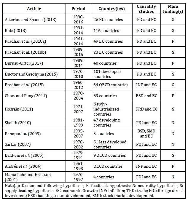
Since it’s such a wide and interesting subject to study, many researchers focus their attention on economic growth and its connection with all the other economic variables, such as banking sector development, stock market development, inflation, trade, foreign direct investment. In the literature it is possible to find studies with different countries and even economic groups. For each study different variables and time horizons are considered. Therefore, the results are not homogeneous. To better show these mixed findings throughout the literature (Batuo et al., 2018; Ibrahim and Alagidede, 2018; Ouyang and Li, 2018; Menyah et al., 2014; Ono, 2017; Hsueh et al., 2013; Kim et al., 2013; Tang and Chea, 2013), and since its common to create literature tables, and with the inspiration in the work of Pradhan et al. (2015), table 1 below was created as a resume from previous studies. It is known that since Schumpeter (1911), an analysis of the interaction between economic growth and alternatives has been used with safety. Goldsmith (1969), McKinnon (1973) and Shaw (1973) focus on the link between financial sector development and economic growth. While Lucas (1988) shows the financial sector only for economic growth. However other studies like Liu and Hsu (2006), Li (2007), Cole, Moshirian and Wu (2008), Rousseau and Yilmazkuday (2009) or Montes and Tiberto (2012), stress that in the long-run, stock market development is key in fostering economic growth. The use of the inflation variable in studies on economic growth are common. Authors such as Boujelbene and Boujelbene (2010); Barro (2013); and Jalil, Tariq, and Bibi (2014) defend that controlled and stable inflation promotes business and investment decisions. So, it’s obvious that inflation and stock market development are related. According to the vast literature, it is difficult to identify whether it is economic growth that drives the other variables (e.g. inflation, trade liberalization, foreign direct investment, banking sector development, stock market development) or, if it’s the variables that drive economic growth. With the support of empirical / mathematical analysis, it’s possible to identify these relationships. Thus, it’s also possible to categorize them in terms of the causal relationship between the variables, in four hypotheses, namely:
i) Neutrality hypothesis – when there is no causality between variables, means that the variables are independent of each other;
ii) Supply-leading hypothesis – when exists unidirectional causality between variables, means causality running from variables to economic growth;
iii) Demand-following hypothesis – when exists unidirectional causality between variables, means causality running from economic growth to one or more variables; and
iv) Feedback hypothesis – when there is a bidirectional causality between variables, means that the causality runs in both directions.
In Table 1, we highlight studies where European countries were analysed. The studies show a statistically significant relationship between the causality of the various variables observed (among them: inflation, trade, foreign direct investment, banking sector development, stock market development and economic growth).
Table 1: Resume of the studies on causality with economic growth
Table 1, shows that the relationship between economic growth and other economics variables. Several authors show a great concern with the topic, since it has been extensively studied in recent years. Among the countries and group of countries studied, researchers found several directions in causality relationship between the variables.
Data and Methodology
To test the relationship between economic growth, banking sector development and stock market development, other control variables were added, namely: inflation, economic and financial openness, so to detect the causality between variables, the estimation is realized by using a Panel Vector Auto-Regressive model (see Abrigo and Love 2015). Next, the data used in this paper are presented and this section is finished by revealing details of the econometric method used.
Data
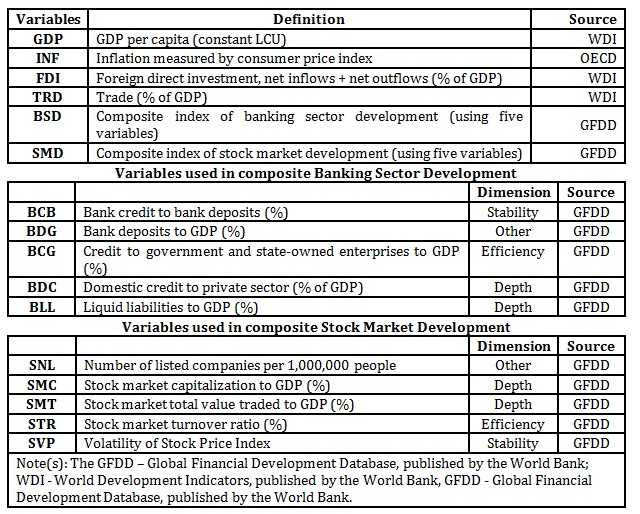
The data come from two large international databases (World Bank and OCDE – Organisation for Economic Co-operation and Development). The twelve European countries sectioned are: Austria, Belgium, Finland, France, Germany, Greece, Ireland, Italy, Luxembourg, Netherlands, Portugal and Spain. The time horizon is restricted to the available data (from 1990 to 2015). The three main reasons to use these selected countries is the fact that they all are European countries with similar culture and history, they all suffered from economic and political changes along the analyses period, changes like joining the Monetary Union, officially called the euro area, and finally because almost all of them suffered the subprime crises (more depth crises in Greece and Portugal with the need of foreign assistance from the International Monetary Fund (IMF) that caused serious damage to the financial markets and infected the real economy. Table 2, shows the description of the variables, the variables used to create the composite of stock market development and banking sector development.
Table 2: Variables description
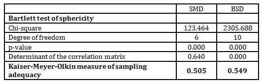
The robustness of the composite index Banking Sector Development (BSD) was verified by the application of Bartlett’s test for sphericity (Bartlett, 1950) and Kaiser-Meyer-Olkin of sampling adequacy (Kaiser, 1970), and table 3 presents the results of the test.
Table 3: Construction of variables
The Kaiser-Meyer-Olkin sampling adequacy measure indicates values above 0.500, so it’s possible to apply the PCA. In the case of the Bartlett’s test for sphericity, the null hypothesis was rejected with a p-value less than 5% (0.000). Also shows a good result of Chi-square and finally reveals that the variables are significantly correlated. Note, the variable SMT was not accepted in the PCA of the Stock Market Development.
Methodology
In this study is applied a technique that combines the regular VAR approach that treats as endogenous all the variables in the system, with the unobserved individual heterogeneity from a panel-data approach (Grossmann et al., 2014). The application of a Panel Data Vector Auto-Regressive model was developed by Love and Zicchino (2006), and used the same methodology. The mentioned model, a first-order PVAR, uses an equation stated as follows in equation 1:
A technique applied by Love and Zicchino (2006) called “Helmert Procedure” (Arellano and Bover, 1995), to solve the problem of fixed effects correlated with the regression related to delays of the dependent variables, usually average differentiation procedure is used to eliminate fixed effects, is also used in the model to avoid the occurrence of biased coefficients. Table 4 presents the descriptive statistics and cross-sectional dependence
Descriptive statistics and cross-sectional dependence
Through table 4, it’s possible to verify that in all variables exists the presence of cross-sectional dependence. The result the statistics of the Inflation Factor of Variance (VIF) shows that multicollinearity is a problem if it is greater than 10. This statistic must be established at the beginning of the estimation in order not to compose the model. Our result shows an average of 1.11 that confirms that multicollinearity is not a problem. Apart from that, Hausman test was performed to determine whether fixed effects. We result are: Chi2 = 16.10 with Prob > Chi2 = 0.0066.and Chi2 = 25.30 with Prob > Chi2 0.0001 in the robust version (sigmamore). Finally, the pvarsoc function of the stata was used to indicate the ideal number of lags. Assuming 1 lag as ideal indicated that MBIC (-279.091), MAIC (-58.1298) and MQIC (-147.86) criteria values. Observation: in results the lowest values indicate the number of lags. It is important to point out the existence of a structural brake on the panel that does not allow capturing the unit root, i.e. the test doesn’t confirm the real stationary effect of the variables, so it was not performed.
Empirical Results and Discussion
In the previous section 3, a preliminary analysis was performed to verify if the PVAR model was the most appropriate. Thus, it was confirmed that the PVAR test was the most appropriate to analyse this nexus between the variables. Note that the PVAR model was estimated using one lag and that all variables are in natural logarithms in their first differences (except inflation which is an index). The Generalized-Method-of-Moments (GMM) was used in the estimation PVAR. In table 6, it is possible to see the test results, after the insertion of the dummies variables to control the shocks and make the model stable and consistent. Just a note that initial a PVAR test was conducted without the presence of the shocks as presented in table 5, but the model was not stable, and not valid to realize the test, so it’s necessary and important the use of shocks in the model.
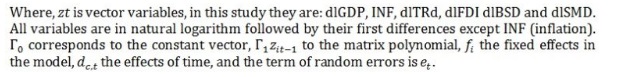
Table 5: Results PVAR and Granger causality without shocks
Despite a PVAR test not valid (without the presence of shocks), and beside the presence of strong endogeneity in the model it’s still possible to make a quick look to table 5 to analyse the relations between variables. Refer that excluded variable does not Granger-cause equation variable is the null hypothesis of the test. First, it’s possible to verify that exists only one bidirectional causality (feedback hypothesis) between variables but at different level of statistical significance, from dlGDP to dlBSD at 1%, and from dlBSD to dlGDP at 5%. However exists a unidirectional causality (supply-leading hypothesis) between: (i) dlGDP to dlBSD; (ii) INF to dlGDP and INF to dlBSD; (iii) dlFDI to dlGDP and dlFDI to dlBSD; (iv) dlTRD to dlGDP and dlTRD to dlBSD; (v) dlSMD to dlGDP and dlSMD to dlBSD, statistical significance at 1% level, also with unidirectional causality but at 5% level of statistical significance it’s possible to find: (i) dlFDI to dlTRD; (ii) dlBSD to dlGDP.
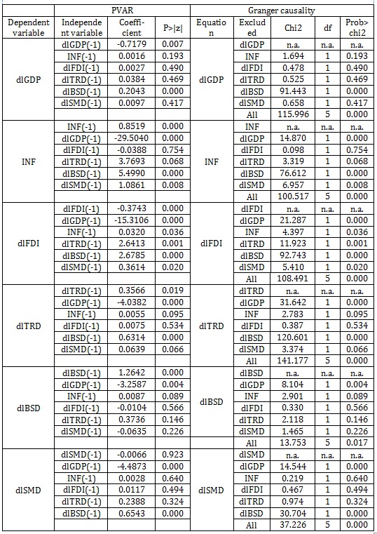
So, the variable with less causality relationship is dlGDP, dlBSD and dlSMD, so if the model was possible to conduct our two main variables will not have many relations with the economic growth. The Eigenvalue test is shown in figure 1, and the results indicate the instability in the model.
Figure 1: Eigen value stability condition without shocks
Despite the strong presence of endogeneity in the model, the instability on it suggests that exist some shocks that need to be controlled in a way that is possible to get a stable model. The dummies variables, impulse and shift, were used to absorb outliers and structural impacts and were applied to year 2001 and for the year 2008 – 2010, respectively. It is important to highlight the use of dummies tool in this paper, to capture the effects of two main situations: (i) integration of the countries in the Monetary Union, because for all of them it was necessary to have monetary stability (relevant for integration); issues created by the physical change of the currency and etc.; (ii) economic distortion caused by the subprime crises which leads to foreign assistance in some countries. In table 6, show the results of PVAR with control of the shocks.
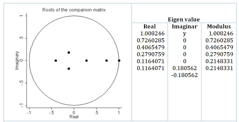
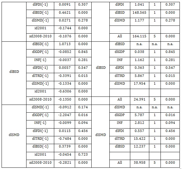
Table 6: Results PVAR and Granger causality with shocks
The null hypothesis of the test is that excluded variable does not Granger-cause equation variable. Therefore, according to table 6 the relations between variables show that there exists a bidirectional causality (feedback hypothesis) between: (i) dlGDP and TRD; (ii) INF and dlSMD; (iii) dlTRD and dlBSD; (ii) dlBSD and dlSMD, statistical significance at 1% level, except from INF to dlSMD and from dlBSD do dlTRD both statistical significance at 5% level and at 10% statistical significance level dlSMD to INF. It also shows that there exists a unidirectional causality (supply-leading hypothesis) between: (i) dlGDP to dlBSD; (ii) INF to dlGDP and INF to dlBSD; (iii) dlFDI to dlGDP and dlFDI to dlBSD and to dlSMD; (iv) dlSMD to dlGDP and dlSMD to dlTRD, statistical significance at 1% level, except from INF to dlGDP, from dlFDI to dlSMD and from dlSMD to dlGDP statistical significance at 5% level. And finally, no causality between: (i) dlGDP to INF, dlFDI and dlSMD; (ii) INF to dlFDI and dlTRD; (iii) dlFDI to INF and dlTRD; (iv) dlTRD to INF, dlFDI and dlSMD; (v) dlBSD to dlGDP, INF and dlFDI; and (vi) dlSMD to dlFDI. So, the variable with less causality relationship is dlGDP, dlTRD and dlBSD, if we look at two of these measures (dlTRD and dlBSD), it’s possible to identify that the European single market can be one of the reasons to reduce these relationships. On the other side, the variable with more causality connexion is dlSMD; this can be explained by the fact that the stock market sector has an important economic role in developed economies. In resume, it is possible to mention that inflation, foreign direct investment, trade and stock market development collaborate to economic growth.
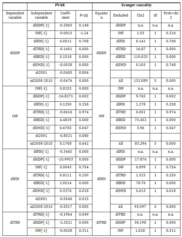
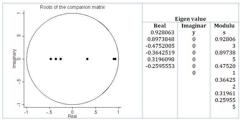
A stability test was also conducted to check the estimations validation (Lütkepohl, 2005). The results satisfy stability condition, because all eigenvalues are inside the circle unit. The eigenvalue test shows the real, imaginary and modulus values, details under figure 2.
Figure 2: Eigen value stability condition with shocks
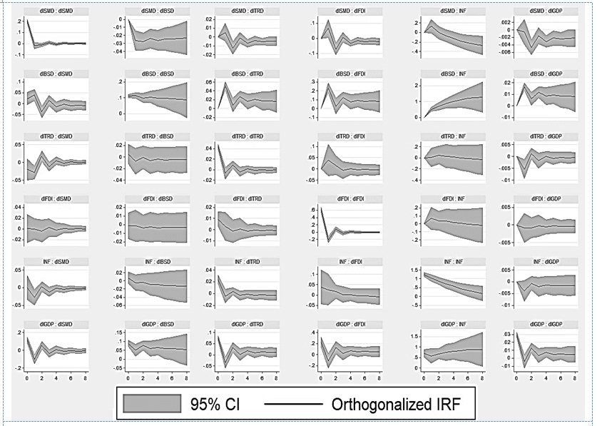
A good estimation of the PVAR model passes through three moments that were executed in this article: the accomplishment of the diagnostic tests before estimating the model, the execution of the model and finally tests of robustness of the estimation. With the results of the impulse-response function presented in figure 3, it’s possible to verify by a graphical analysis how the variables react to an exogenous shock, and the periods it needs to return to is equilibrium. The first interpretation we can redraw from the graph is that almost all variables recover from the shock in a four years period. Second is possible to identify dlBSD as the variable more stability in response to the shocks in all other variables and that dlSMD is a variable that have an intense response on the beginning of the shock, but after a four years period stabilizes. Third is possible to verify that dlTRD and dlFDI after the shock occur, when stabilized, both stay on a lower level than before.
Figure 3 : Impulse and response
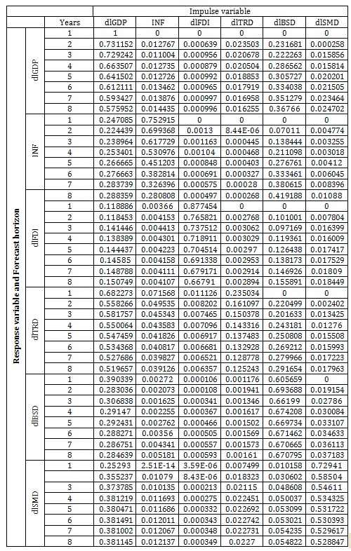
The Forecast-Error Variance Decomposition (FEVD) was performed (table 7) so that it was possible to analyse how the variables react to exogenous shocks (Marques, Fuinhas and Marques, 2013). Common practice in macroeconomic studies (Charfeddine and Kahia, 2019; Jawadi et al., 2016; Brana et al., 2012), even in the study conducted by Jawadi et al. (2016) it was used a dummy to control the economic crises so that it was possible to have a stable model. Table 7: Forecast-error variance decomposition
Table 7: Forecast-error variance decomposition
Observing table 7, it’s possible to identify that the biggest variations in the variables occur when the shock is over themselves. With more detail and watching at a four years period after the shock (when by default the variables starts to stabilize), it’s possible to identify: (i) dlGDP variable auto explains about 66,4% of the FEVD; (ii) a shock to INF, variable auto explains 53,1%; (iii) a shock to dlTRD variable auto explains 14,3%; (iv) a shock to dlBSD variable auto explains 67,4%; (v) a shock to dlSMD variable auto explains 53,4%. So, the variable with less auto explanation is the dlTRD because in a scenario of a shock to dlTRD the variable with more reaction is the dlGDP this may be explained with the fact that the economies under study perform an enormous trade (goods and services) relation between them (all European countries). Its also important to mention that dlBSD plays an important role in the FEVD when compared with dlSMD, by norm have an equal or bigger reaction to the shock, even when the shock happens to dlSMD, this may occur because the economies under study are more banking sector dependent that stock market dependent, so this make them more volatile to shocks in dlBSD.
According to the above results dlTRD have a feedback hypothesis with dlGDP and with dlBSD, so it’s important that the European countries try to attract foreign direct investment from outside Europe so that they can maintain a wealth and sustainable growth and be less vulnerable to crises, as is it possible to. The way how the economic agents and the governments interact in develop countries with a strong dependence from the banking system, like the case under study were the variable dlBSD represent feedback hypothesis between dlTRD and dlSMD should aim as a principal objective the social well-being and create measures between public and private agents to reach this goal. Even solid markets and stable financial systems can be vulnerable to the negative effects generated by a global crisis similar to the one experienced in 2008. This vulnerability can be reduced or at least minimized if the policies encourage the agents to diversify the investments and the areas of expertise e.g. investments in tourism, so these new areas of expertise should be boost in a way to recover economies from crises periods. Sustainable growth now a days is a global concern, so the developed countries should encourage the financial system to make contributions to this major concern by helping with social projects, sustainable development, income inequality and with the economy in general. Corroborate with the suggestion of Charfeddine and Kahia (2019) that the banking operations should support green energy projects and low carbon emissions projects. In the next section, we show the conclusion and contribution of this study to the economy. The study also suggests a topic for future studies.
Conclusion
In this study we estimated an Auto-Regressive Vector Panel model for a panel of twelve European countries and a time span from 1990 to 2015. The relationship between economic growth and banking sector development and stock market development was analysed. By using a Principal Component Analysis mode, it was possible to create two new measures, one for banking sector development and the other for stock market development, which includes four financial dimension measures: depth, efficiency, stability and other; this way it was possible to realize the study with composite to identify specific financial markets (bank and stocks). After estimation the three hypotheses of this study were verified and confirmed. The model is endogenous; the shocks (introduction of the euro and the subprime financial crisis) are statistically significant and should be considered in future studies; and finally, banking sector development and stock market development have significant statistical relationships with each other when the shocks in the economy are controlled. The estimation results respond to the previous hypotheses according the existence of feedback hypothesis between economic growth and economic openness, (i.e. governments should implement a well-supported economic openness, promoting economic trade – import export of goods and services). However, it also shows neutrality hypothesis between economic growth to stock market development and financial openness. It denotes also that inflation (INF), foreign direct investment (FDI) and stock market development (BSD) granger-cause economic growth. So, to promote economic growth, the policies should induce a healthy and sustained external relation to help economic openness, also some good financial resources to support a good stock market development because there is a relationship with economic growth. As a main contribution, it’s possible to refer to the set of countries chosen, because they are a homogenous group with the same currency and similar economic shocks like the subprime crises, which had a huge impact over the economy, and to refer to the new aspect of including the economic and financial openness in the study to interrelate with the financial development. For future studies, it is important to get a set of countries with different economic spheres to confirm the impact of financial development and economic openness over the economy. Another interesting suggestion would be the individual analysis of the countries to be able to compare them with the results obtained in the studies that analyse the panel countries.
Acknowledgments
The financial support of the NECE – Research Unit in Business Science and Economics, sponsored by the FCT – Portuguese Foundation for the Development of Science and Technology, Ministry of Science, Technology and Higher Education, project UID/GES/04630/2019, is acknowledged. Research supported by: CEFAGE, R&D unit funded by the FCT – Portuguese Foundation for Science and Technology, Ministry of Science, Technology and Higher Education, project UID/ECO/04007/2019.
Abrigo, MR and Love, I. (2015), Estimation of Panel Vector Autoregression in Stata: a Package of Programs. 21. International Panel Data Conference [Online], [Retrieved September 09, 2018], http://paneldataconference2015.ceu.hu/Program/Michael-Abrigo.pdf.
Andrés, J., Hernando, I. and Lopez-Salido, D. (2004), ‘The Role of the Financial System in the Growth–inflation Link.’ European Journal of Political Economy, 20 (4), 941–961.
Arellano, M. and Bover, O. (1995), ‘Another look at the instrumental variable estimation of error components models.’ Journal of Econometrics, 68, 29-51.
Asteriou, D. and Spanos, K. (2018), ‘The relationship between financial development and economic growth during the recent crisis: Evidence from the EU.’ Finance Research Letters, (in press).
Baldwin, R., Braconier, H. and Forshid, R. (2005), ‘Multinationals, endogenous growth, and technological spillovers: theory and evidence.’ Review of International Economics, 13, 945–963.
Barro, RJ. (2013), ‘Inflation and economic growth.’ Annals of Economics and Finance, 14 (1), 121-144.
Barro, RJ. and Sala-i-Martin, X. (1995) Economic Growth, McGraw Hill, New York.
Bartlett, MS. (1950), ‘Tests of significance in factor analysis.’ British Journal of Mathematical and Statistical Psychology, 3(2), 77-85.
Batuo, M., Mlambo, K. and Asongu, S. (2018), ‘Linkages between financial development, financial instability, financial liberalisation and economic growth in Africa.’ Research in International Business and Finance, 45, 168-179.
Beck, T. and Levine, R. (2004), ‘Stock Markets, banks, and growth: Panel evidence.’ Journal of Banking and Finance, 28(3), 423-442.
Bertocco, G. (2008), ‘Finance and development: is Schumpeter’s analysis still relevant?’ Journal of Banking & Finance, 32 (6), 1161–1175.
Boujelbene, T. and Boujelbene, Y. (2010), ‘Long Run determinants and short run dynamics of inflation in Tunisia.’ Applied Economics Letters, 17(13), 1255-1263.
Brana, S., Djigbenou, ML. and Prat, S. (2012), ‘Global excess liquidity and asset prices in emerging countries: A PVAR approach.’ Emerging Markets Review, 13(3), 256-267.
Charfeddine, L., and Kahia, M. (2019), ‘Impact of renewable energy consumption and financial development on CO2 emissions and economic growth in the MENA region: A panel vector autoregressive (PVAR) analysis.’ Renewable Energy, 139, 198-213.
Chow, WW. and Fung, MK. (2011), ‘Financial development and growth: A clustering and causality analysis.’ Journal of International Trade and Economic Development, 35(3), 1–24.
Cole, RA., Moshirian, F. and Wu, Q. (2008), ‘Bank stock returns and economic growth.’ Journal of Banking and Finance, 32(6), 995–1007.
Ductor, L. and Grechyna, D. (2015), ‘Financial development, real sector, and economic growth.’ International Review of Economics & Finance, 37, 393-405.
Durusu-Ciftci, D., Ispir, M. and Yetkiner, H. (2017), ‘Financial development and economic growth: Some theory and more evidence.’ Journal of Policy Modeling, 39, 290-306.
Fink, G., Haiss, P. and Vuksic, G. (2009), ‘Contribution of financial market segments at different stages of development: Transition, cohesion and mature economies compared.’ Journal of Financial Stability, 5(4), 431-455.
Fischer, S. (1993), ‘The role of macroeconomic factors in growth.’ Journal of Monetary Economics, 32(3), 485-512.
Goldsmith, RW. (1969) Financial Structure and Development, Yale University Press, New Haven,Connecticut.
Holtz-Eakin, D., Newey, W. and Rosen, H. (1988), ‘Estimating Vector Autoregressions with Panel Data.’ Econometrica, 56, 1371-1395.
Hossain, MS. (2011), ‘Panel estimation for CO2emissions, energy consumption, economic growth, trade openness, and urbanization of newly industrialized countries.’ Energy Policy, 39(11), 6991–6999.
Hsueh, S., Hu, Y. and Tu, C. (2013), ‘Economic growth and financial development in Asian countries: A bootstrap panel granger causality analysis.’ Economic Modelling, 32(3), 294–301.
Ibrahim, M. and Alagidede, P. (2018), ‘Nonlinearities in ?nancial development–economic growth nexus: Evidence from sub-Saharan Africa.’ Research in International Business and Finance, 46, 95-104.
Jalil, A., Tariq, R. and Bibi, N. (2014), ‘Fiscal deficit and inflation: New evidences from Tunisia.’ Journal of Policy Modelling, 36(1), 883-898.
Jawadi, F., Mallick, SK. and Sousa, RM. (2016). ‘Fiscal and monetary policies in the BRICS: A panel VAR approach.’ Economic Modelling, 58, 535-542.
Kaiser, H F. (1970), ‘A second generation little jiffy.’ Psychometrika, 35(4), 401–415.
Kim, S., Lim, H. and Park, D. (2013), ‘Does Productivity Growth Lower Inflation in Korea?’ Applied Economics, 45 (29), 2183-2190.
Levine, R. (1997), ‘Financial development and economic growth: views and agenda.’ Journal of Economic Literature, 35 (2), 688–726.
Levine, R. and Zervos, S. (1998), ‘Stock markets, banks and economic growth.’ American Economic Review, 88(3), 537-558.
Li, K. (2007), ‘The growth in equity market size and trading activity: An international study.’ Journal of Empirical Finance, 14(1), 59–90.
Liu, W. and Hsu, C. (2006), ‘The role of financial development in economic growth: The experiences of Taiwan, Korea and Japan.’ Journal of Asian Economics, 17(1), 667–690.
Liu, X. and Sinclair, P. (2008), ‘Does the linkage between stock market performance and economic growth vary across greater China.’ Applied Economics Letters, 15(7), 505–508.
Love, I. and Zicchino, L. (2006), ‘Financial development and dynamic investment behaviour: evidence from panel VAR.’ The Quarterly Review of Economics and Finance, 46(2), 190-210.
Lucas, RE. (1988), ‘On the mechanics of economic development.’ Journal of Monetary Economics, 22, 3–42.
Lütkepohl, H. (2005) New Introduction to Multiple Time Series Analysis, Springer Science & Business Media, Berlin, Heidelberg, New York.
Mankiw, NG., Romer, D. and Weil, DN. (1992), ‘A contribution to the empirics of economic growth.’ Quarterly Journal of Economics, 107(2), 407-437.
Manuchehr, I. and Ericsson, J. (2001a), ‘On the causality between foreign direct investment and output: a comparative study.’ The International Trade Journal, 15(1), 1–26.
McKinnon, RI. (1973), Money and Capital in Economic Development, Brookings Institution Press, Washington, DC.
Menyah, K., Nazlioglu, S. and Wolde-Rufael, Y. (2014), ‘Financial development, trade openness and economic growth in African countries: New insights from a panel causality approach.’ Economic Modelling, 37(2), 386–394.
Montes, GC. and Tiberto, BP. (2012), ‘Macroeconomic environment, country risk and stock market performance: Evidence for Brazil.’ Economic Modelling, 29(3), 1666–1678.
Nguyen, TT. and Wang, K. (2010), ‘Causality between housing returns, inflation and economic growth with endogenous breaks.’ Journal of Chinese Economic and Business Studies, 8(1), 95-15.
Ono, S. (2017), ‘Financial development and economic growth nexus in Russia.’ Russian Journal of Economics, 3(3), 321-332.
Ouyang, Y. and Li, P. (2018), ‘On the nexus of ?nancial development, economic growth, and energy consumption in China: New perspective from a GMM panel VAR approach.’ Energy Economics, 71, 238-252.
Panopoulou, E. (2009), ‘Financial variables and euro area growth: A non-parametric causality analysis.’ Economic Modelling, 26(6), 1414-1419.
Pradhan, RP., Arvin, MB. and Bahmani, S. (2015), ‘Causal nexus between economic growth, inflation, and stock market development: The case of OECD countries.’ Global Finance Journal, 27, 98-111.
Pradhan, RP., Arvin, M. and Bahmani, S. (2018a), ‘Are innovation and ?nancial development causative factors in economic growth? Evidence from a panel granger causality test.’ Technological Forecasting & Social Change, 132, 130-142.
Pradhan, RP., et al. (2018b), ‘Endogenous dynamics between innovation, financial markets, venture capital and economic growth: Evidence from Europe.’ Journal of Multinational Financial Management, 45, 15-34.
Romer, D. (1998), ‘A new assessment of openness and inflation: reply.’ The Quarterly Journal of Economics, 113 (2), 649-442.
Rousseau, PL. and Yilmazkuday, H. (2009), ‘Inflation, financial development, and growth: A trilateral analysis.’ Economic Systems, 33(4), 310–324.
Ruiz, JL. (2018), ‘Financial development, institutional investors, and economic growth.’ International Review of Economics & Finance, 54, 218-224.
Sarkar, P. (2007), ‘Does Foreign Direct Investment Promote Growth? Panel data and Time Series Evidence from Less Developed Countries, 1970-2002.’ MPRA – Munich Personal RePEc Archive, 6(5176), 1–23.
Schumpeter, JA. (1911) The Theory of Economic Development, Harvard University Press, Cambridge, Massachusetts.
Shahbaz, M. (2012), ‘Does trade openness affect long run growth? Cointegration, causality and forecast error variance decomposition tests for Pakistan.’ Economic Modelling, 29(6), 2325–2339.
Shaikh, FM. (2010), ‘Causality Relationship between Foreign Direct Investment, Trade and Economic Growth in Pakistan.’ Asian Social Science, 1(4), 82-89.
Shaw, ES. (1973) Financial Deepening in Economic Development, Oxford University Press, London.
Tang, TC. and Chea, R. (2013), Export-Led Growth in Cambodia: An Empirical Study. Discussion Paper, no. 03/13, Monash University Sunway Campus, Selangor.
Yartey, CA. (2008), The Determinants of Stock Market Development in Emerging Economies: Is South Africa Different. IMF Working Paper, no. WP/08/32 (pp. 1-31), Washington DC: International Monetary Fund.
Yucel, F. (2009), ‘Causal relationship between financial development, trade openness, and economic growth: The case of Turkey.’ Journal of Social Sciences, 5(1), 33-42.
Notes
Kaiser-Meyer-Olkin: Result value between 0 and 1 and if the output is below 0.5 the PCA must not be applied.
The Bartlett’s: The null hypothesis is that variables are not intercorrelated