The Dynamics of The Romanian Electronics Trade Flows – A Gravity Model Approach

Introduction

Romanian trade flows with electronics in 2001-2018 period – brief overview

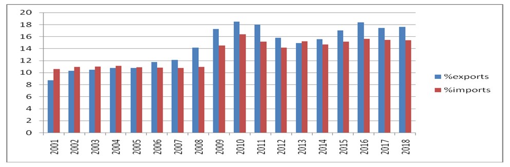
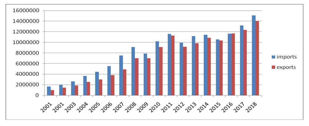
Electronics are among the most important Romanian exports, as well as imports in 2001 – 2018 period. The value of the exported electronics was 14 times greater in 2018 than in 2001, while the import value was 9 times greater, yet except for year 2016, when exports surpassed imports, Romania remained a net importer of electronics. Germany was the main trading partner.  In the top 10 electronics’ importers, there were mainly EU countries and the electronics’ imports came also from EU countries, with the exception of China.

Fig. 1: The share of electronics in all the exported and imported goods

Source: Author’s figure based on data from https://www.trademap.org/tradestat/Product_SelCountry_TS.aspx?nvpm

Fig. 2: The value of electronics imports and exports in US dollars in the period 2001-2018

Source: Author’s figure based on data from https://www.trademap.org/tradestat/Product_SelCountry_TS.aspx?nvpm

Literature Review

The gravity model was developed independently by Tinberger (1962) and by Poyhonen (1963), although a gravity theory was previously developed by Adam Smith, refering to a proportional relationship between the economic size and distance (Elmslie, 2018). Over more than 50 years, the gravity model became the most successful model for international trade and it is often labeled as the workhorse of the research in this field. The initial gravity model is based on Newton’s gravity law: the force between two particles is directly proportional with their mass and inversely proportional with the square of the distance between them. The translation for Newton’s law of universal attraction goes like this: the trade flows between two countries is positively influenced by their economic size and negatively influenced by the distance between them. What does the economic size mean? Could be GDP, GNI (formally GNP), GDP per capita, population, income, GDP per capita. What does distance mean? In the first place, it was simply the geographical distance between the capitals of the two countries, but later it became a proxy for trade costs, transport costs, taxes and tariffs, transaction costs, communication costs, cultural distance, and country familiarity.

For more than a decade, the gravity model was just a successful empirical model with no solid theoretical base. It was in 1979 when Anderson developed a solid theoretical foundation for the gravity model based on Armington’s assumption “Goods are differentiated by their country of origin” and introduced the term economic distance. Bergstrand added price variables in 1985. The Helpman and Krugman model was developed in 1985 to mainly explain the intra-industry international trade. Bergstrand (1985, 1989) considered a Heckscher-Ohlin model, including a monopolistic competition with differentiated products to develop the theory of gravity. If Helpman, Krugman and Bergstand were critics to Heckscher and Ohlin, in 1998, Deardorff was critical with respect to the critics of Helpman, Krugman and Bergstand and reevaluated the Heckscher-Ohlin model. According to this model, countries that are close to each other will tend to trade more, while countries which are far from one another will trade even less than the predicted trade. Evenett and Keller (2002) tested both models and concluded that both models are a theoretical base for the gravity model, but the Heckscher-Ohlin model should be preferred from an empirical point of view. All the models have an explanatory power of at least 80%. 

Regarding the relationship between the gravity equation and the models which generated the equation:

–  The gravity equations fit in with the Heckscher-Ohlin model of inter-industry, as well as with the Helpman – Krugman – Markusen model of intra industry trade (Berstrand, 1989).

– The gravity equation is a reduced form from a partial equilibrium subsystem (Bergstrand, 1985).

– The gravity equation could be generated by a model with incomplete specialization and trade costs (Haveman and Hummels, 2004).

– The estimates from the gravity equation could be different when  heterogeneity is considered (Tzouvelekas, 2007).

The debate on the best model is not over yet: if all the random components of the model are homoskedastic, the Helpman-Melitz-Rubinstein model works better (Santos Silva and Tenreyro, 2009).

The Pros of the gravity model:

• Has a better overall performance compared to radiation models (Masucci, et al., 2013).
• It’s perfectly applicable to a single country case (Sohn, 2005).
• Was used for over than 50 years to analyze the impact of the globalization factors on the bilateral trade (Bergstrand and Egger, 2009).
• The augmented gravity model including Linder hypothesis is better suited for tourism flows than the traditional gravity model (Tamaș, 2019).
• Explains the financial transactions in the same manner as the trade with goods (Portes and Rey, 2005).
• Could be applied to the International Trade Network (Fagiolo, 2010).
• The trade with homogeneous goods is better described by the gravity model (Feenstra, Markusen & Rose, 2001).
• The gravity model could be used to study the traffic flows between cities (Jung, Wang & Stanley, 2008).
• The more technologically complex and intense the industries are, the larger the gravity strenghth is (Keller and Yeaple, 2009).
• The inter cities’ communications are explained by the gravity model (Krings, et al., 2009).

The Cons of the gravity model:

• Performs poorly for bilateral trade with parts and components (Baldwin & Taglioni, 2010).
• The traditional gravity model estimates are not reliable in analyzing the East-West trade potential (Breuss and Egger, 1999).
• The results of the gravity model for the potential trade are highly sensitive on the country heterogeneity (De Benedictis and Vicarelli, 2005).
• The use of the gravity model for the trade policies is severely limited (De Benedictis and Vicarelli, 2009).

The major problems of the gravity model are related to the heteroskedasticity in the trade data and the existence of the zero flows (Gómez-Herrera, 2013). The zero trade may occur if the trade volume or value is too small or if the firms of the exporting country are not competitive enough for the customers in the importing country (Anderson, 2011). Zero values are very common in trade data and omitting them could lead to omitting important information (Shepherd, 2008). Zero values should not be neglected because of the information they may contain (De Benedictis and Taglioni, 2011). Treating zero trade flows properly is important from both a statistical and an economical perspective (Haq, Meilke and Cranfield, 2010). Among all the solutions to deal with the zeroes (omitting the zeroes, various Tobit estimations, truncated regression, substitutions for zeroes), omitting the zeroes from the sample leads to the most acceptable results (Linders and de Groot, 2006).

Methodological issues:

• The linear approximation method can have lower average absolute comparative static errors (Baier and Berstrand, 2009).
• The simple least squares estimates outperform the generalized method of moments for dynamic panels (Bun and Klaassen, 2002).
• The fixed effects estimator is similar to a dynamic OLS (Fidrmuc, 2009).
• The Standard Poisson model, seen as an alternative to log normality assumption, is vulnerable to excess zero flows and over dispersion (Burger, van Oort and Linders, 2009).
• The Poisson Pseudo-Maximum Likelihood estimator solves the heteroscedasticity bias problem only when it is the only problem, and fails to do so when the heteroscedasticity bias is combined with frequent zeroes (Martin and Pham, 2008).
• For small samples, the performances of the Poisson Pseudo-Maximum Likelihood estimator and of the Feasible Generalized Least Squares estimator are similar (Martinez Zarzoso, 2013) (Westerlund and Wilhelmsson, 2009).
• The Poisson Pseudo-Maximum Likelihood estimator leads to significant differences compared to traditional estimators (Santos Silva and Tenreyro, 2006).
• The Poisson Pseudo-Maximum Likelihood estimator is still robust for large proportions of zeroes (Santos Silva and Tenreyro, 2011).
• The nonparametric cross section estimates are more stable than the OLS cross section estimates (Baier and Bergstrand, 2009).
• The Anderson-Van Wincoop’s multilateral trade resistance factor, which works with cross section data, could be adaptive to panel data, as well as using time variant country dummies (Baldwin and Taglioni, 2006).
• The omission of interactions might lead to biased estimates (Baltagi, Egger and Pfaffermayr, 2003).
• Panel estimations should be considered instead of cross section estimations (Egger, 1999) and fixed effects should be preferred to random effects (De Benedictis and Taglioni, 2011).
• A proper gravity equation should include time invariant bilateral interactions (Egger and Pfaffermayr, 2003).
• The gravity equations perform better in explaining the trade among the industrial nations (Evenett and Keller, 2002).
• Spatial autocorrelation and heterogeneity are affected by the bias introduced by a logarithmic scale in the gravity equation (Porojan, 2001).
• The log linearity of the gravity equation could be replaced by Box Cox transformations (Sanso, Rogelio and Sanz, 1993).

Among all the trade determinants, the income or the GDP plays a special role. Income growth explains 67% of the trade flows (Baier and Bergstrand, 2001). Income differences, exchange rates and infrastructure are among the most important determinants of bilateral trade flows (Martínez-Zarzoso and Nowak-Lehman, 2003). GDP per capita and common membership positively influence the wine trade flows (Tamaș, 2017). Income, population, production capacity and distance are the determinants of the meat trade (Karemera, et al. 2015). There is a positive robust correlation between the investment share and the ratio of international trade to GDP (Levine and Renelt, 1992). The trade openness of a country is inversely proportional with the size of the country (Siliverstovs and Schumacher, 2008). The trade volumes depend on the trading partners and are smaller for pairs of less developed countries compared to pairs of developed and less developed countries (Helpman, Melitz and Rubinstein, 2008). Usually, GDP coefficients are between 0.5 and 1.5.

Distance is an important determinant of the trade flows. The negative effect of the distance on the trade flows has been high since the middle of the century (Head, 2008). The absolute value of the distance increased over the time (Brun, et al., 2005). The distance impact is larger when OLS is used (Siliverstovs and Schumacher, 2008). The existing measure for the distance between two countries overestimates the distance effect on the trade flows (Keith and Mayer, 2002). The geographical distance is more important for services trade than it is for goods trade (Kimura and Lee, 2004). Distance has a larger effect on the number of exporting firms than on export sales (Lawless, 2010). Internal distance has an impact 10 times larger than remoteness (Melitz, 2007).

Distance is an imperfect proxy for the trade costs and its effects differ among trading goods (De Benedictis and Taglioni, 2011). Distance combined with common language, common culture and country familiarity play an important role in the gravity model (Deardoff, 1998). The negative impact of the distance on the trade flows could be explained not only by the transport costs, but also by the unfamiliarity of the countries (Grossman, 1996). Usually, distance coefficients are between -0.6 and -1.6.

However, in special cases, distance could have a smaller effect on the trade flows. Exports and imports among the countries from the Gulf Cooperation Council do not depend on the distance because of the development of the transport facilities and the characteristics of the region (Filippini and Molini, 2003). The geographical distance and the cultural distance do not have a significant influence on the Erasmus students flows (Tamaș, 2017). The distance has no statistical effect on non taste dependent products, like software, while for taste dependent products, like movies, it has a similar effect as for goods (Blum and Goldfarb, 2006).

Moreover,  the distance is associated with the trade costs. Transport costs reductions explain 8% of the trade flows, while tariff rate reductions explain 25% of them (Baier and Bergstrand, 2001). The trade costs depend on the size of the country (Baier and Berstrand, 2009). Trade costs vary among countries; developing countries have trade costs 7 times larger than developed countries (Anderson and van Wincoop, 2004). Surprisingly, most country pairs reduce their trade after a multilateral fall in trade costs (Behar and Nelson, 2014). The impact of the trade barriers is reduced by the elasticity of the substitution (Chaney, 2008). A fall in the trade costs increases the trade volumes and the number of firms of the exporting country which enter the trade (Anderson, 2011). Trade costs could be used for the gravity, but also the gravity model could be used to analyze the impact of the infrastructure investments on the trade costs (Egger, 2002).

In relationship with the distance effect, there is also a common border effect. It is not clear why the common border matters as long as distance (Head, 2003). The gravity model produces consistent estimates regarding the average border effect on the trade flows (Feenstra, 2002). The border effect is sensitive regarding the size and the sign of the chosen method (Magerman, Studnicka and Van Hove, 2016). National borders reduce the trade among the industrialized countries by 30% (Anderson and van Wincoop, 2003). Border effects remain large even when the tariffs are very small (Head and Mayer, 2013). Countries that are close to each other have fewer opportunities to develop export opportunities (Stavytskyy, et al., 2019). The most easily transportable industries have no border effect (Keith and Mayer, 2002).

The membership in the same trade agreement has a positive impact on trade flows. The common membership is one of the most used dummies in the gravity model.

The results show that both the EEC and EFTA have experienced a cumulative growth in gross trade creation (GTC), with the GTC of the EEC being substantially greater than the GTC of EFTA (Aitken, 1973). The probability of two countries already having a trade agreement to have another trade agreement with another country is 50 times larger than the probability that any of the first two countries to have another agreement with the third one (Baier and Bergstrand, 2004). The gravity model tends to overestimate the effect of the integration on the trade volumes (Cheng and Wall, 1999). There is no additional trade between Turkey and EU following the Association Act from 1963 and the customs union from 1996 (Antonucci and Manzocchi, 2006). Trade flows are influenced by amity or enmity between countries (Pollins, 1989).

Free Trade Agreements (FTAs) effect: FTAs increase trade flows 4 times. A FTA could double the trade flows between two countries in 10 years (Baier and Bergstrand, 2007). The effects of the FTAs for the less developed countries trade flows (Cambodia, Laos, Myanmar and Vietnam) are negative (Roberts, 2004).

Preferential Trade Agreements (PTAs) effect: foster the trade among the countries in the PTA (Cardamone, 2007).

Regional Trade Agreements (RTAs) effect: increase the trade among their members on the expense of the non members (Carrere, 2006).  RTAs have a positive impact on the bilateral trade (Cipollina and Salvatici, 2010). The RTAs have a larger positive effect on the trade flows for the developed countries compared to the developing countries (Horsewood, 2009). Membership in the same RTA has a positive effect on goods trade, as well as on services trade (Kimura and Lee, 2004). Regional integration may increase the trade flows, but sometimes it leads to a decline (Elliott, 2007).

Similarity seems to have a positive influence on the trade flows. Similarities between countries regarding GDP per capita and population positively influence the trade flows (Miron, Cojocariu and Tamaș, 2019). Similar cultural attributes lead to trade flows increasing (Söderström, 2008). Trade among countries with similar income per capita is more intense (Hallak, 2010). 

Gravity model best fits for countries with similar preferences for traded goods and similar trade costs (Anderson, 1979). The similarities between two countries regarding the capital – labor relationship have an impact on the intra-industry bilateral trade (Bergstrand, 1990). If two countries with similar GDP have a bilateral trade and one of them reaches a higher GDP, the first goods which this country will eliminate from the trade would be the actual goods exported by the other country (Linder, 1961). The Linder hypothesis gains strength since 1990 due to globalization (Choi, 2002). The Linder effect on the bilateral Foreign Direct Investments is larger in industries with greater quality differentiation (Fajgelbaum, Grossman & Helpman, 2011).

Tourists’ flows are determined by the similarities in preference between the origin and the destination country and the climate distance (Lorde, Li and Airey, 2015). Linguistic similarities between the country of origin and the host country have a positive impact on Erasmus students’ flows (Tamaș, 2017). Although Greece and Portugal have similar characteristics, their exports differ because of Greece’s unique geographical position in EU (Papazoglou, 2007).

Other variables were considered over the time, like migration (Migrants stimulate exports, but have no impact on imports (Hatzigeorgiou and Lodefalk, 2015)) or exchange rate (Increasing exchange rate volatility or other things equally is detrimental to trade (Abrams, 1980)). Euro has a positive impact on the overall trade flows (Baldwin and Di Nino, 2006). Increasing exchange rate variability affects bilateral trade flows (Thursby and Thursby, 1987).

Research hypothesis

1. The economic size (measured by GDP) of Romania and the partner countries positively influences the electronics trade flows.
2. The distance (between the countries, as well as within the countries) negatively impacts the electronics trade flows.
3. EU membership positively influences the electronics trade flows.
4. Economic factors, like partners’ inflation, negatively impact the trade flows of a net electronics importer.
5. Trade policy factors, like trade openness (measured as the percentage of trade in the GDP) of the partner countries positively influence the electronics trade flows.
6. Political factors, like stability, positively impact the electronics trade flows.
7. Replacing two variables (the SDINT and the DISTINT), would significantly impact the results.

Data Description and Methodology

The gravity equation:

LNTRADE_t = c₀ + c₁LnGDP_t + c₂LnGDPR_t + c₃LnDIST + c₄LnSDINT + c₅LnINFLATION_t + c₅LnINFLATIONR_t + c₆ LnTRADEOPEN_t + c₇LnTRADEOPENR_t + c₈LnSTABILITY_t + c₉LnSTABILITYR_t + c₁₀EU + c₁₁COMBOR + e_k

Trade_t is the dependent variable, it represents the total values of the electronic bilateral trade between Romania and a partner country in year t, where t takes values from 2001 to 2018.

GDP_t is the GDP of a partner country in year t and GDPR is the GDP of Romania in year t. They both are expected to have coefficients with positive signs and values between 0.2 to 1 (Head, 2003). The data is from https://data.worldbank.org › .

DIST is the distance between the capital cities of Romania and the partner countries. It is expected to have a coefficient with a negative sign and values from -0.6 to -1.6 for dist. The data is from www.chemical-ecology.net  for DIST variable and from www.cepii.fr › pdf_pub  for internal distance. SDINT is the sum of the internal distance of Romania and the partner country. It is expected to have a coefficient with a negative sign and values smaller than those of DIST (Melitz, 2007). DISTINT is the internal distance of the partner country.  The data are from www.cepii.fr › pdf_pub.  The coefficient is expected to have negative signs and smaller values as DIST.

INFLATION_t and INFLATIONR_t are respectively the inflation rates of the partner country and of Romania in year t. A positive sign of the coefficient should have a positive impact on the exports; therefore, a positive impact on the trade flows if the country is a net exporter (Stockman, 1981).

TROPEN_t and TROPENR_t are respectively the trade openness of the partner country and of Romania in year t. It is expected to have a coefficient with a positive sign if the country is a net exporter (Anderson and Neary, 2005). The data is from https://data.worldbank.org › .

STABILITY_t and STABILITYR_t are respectively the indexes for political stability for the partner country and for Romania in year t. It is expected to have a coefficient with a positive sign. The data is from https://www.theglobaleconomy.com › rankings .

EU is a dichotomic variable, taking the value 1 if both Romania and the partner countries are EU members and 0 otherwise. The coefficient should have positive signs and values larger than 1 (Abrams, 1980).

COMBOR is a dichotomic variable, taking the value 1 if both Romania and the partner countries share a common border and 0 otherwise. The coefficient should have positive signs and values around 1 (Head, 2003).

An unbalanced panel approach was used to address the heteroskedasticity issue (Breuss and Egger, 1999). Also, a dynamic panel model was considered for better results (Bun and Klaassen, 2002). The zero flows were omitted in the sample as often, leading to the most acceptable results (Linders and de Groot, 2006). The EViews soft version 8 was used.

Results and Discussions

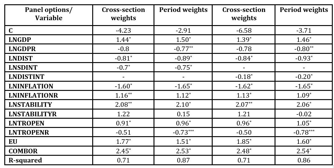
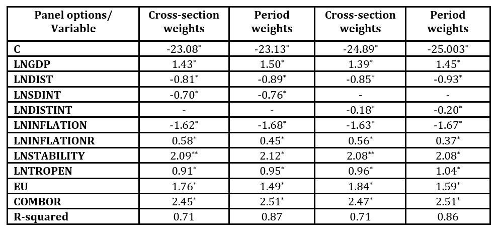
Table 1: The results for the panel regression

Legend statistically significant at 1% ^*, at 5% ^**, at 10%^***

Source: Author’s table based on the outputs

Some of the variables are not statistically significant: STABILITYR and C in either versions, GDPR and TROPENR in the first one.

The coefficients for GDP are between 1.39 and 1.5 for the whole period, which proves that the Romanian trade flows follow a GDP pattern, relaying on the trading partners’ economic size, and that the electronics exports are mainly based on quantity and low prices.

The results for the distance between the countries are in line with the previous studies, between   -0.93 and -0.81. For internal distance, if both Romania and the partner countries are taken into account, the coefficients are from -0.75 to -0.7, but when taking into account only the internal distance for the trading partner, the values are from -0.2 to -0.18.

The trading partners’ inflation negatively impacts the trade flows because it diminishes the buying power of the Romanian trading partners. But the Romanian inflation positively influences mainly the exports, which are based on low prices, making the prices even more affordable.

The political stability of the trading partners strongly and positively influences the trade flows, even more than the trade openness does. On the long run, the Romanian trade openness negatively influences the trade flows, maybe because of the low competitiveness of the products.

As expected, the EU membership has a powerful and positive influence; the values are from 1.51 to 1.85.

The common border has a positive influence; the values are overestimated by the model 5 times in average, which sustains the findings of Keith and Mayer (2002).

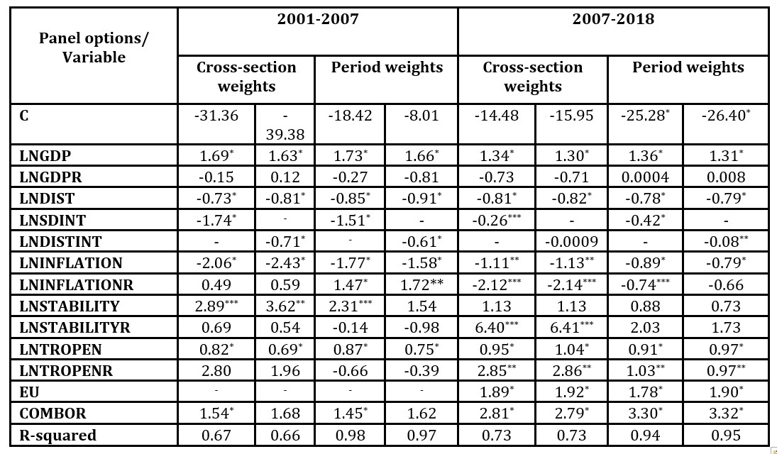
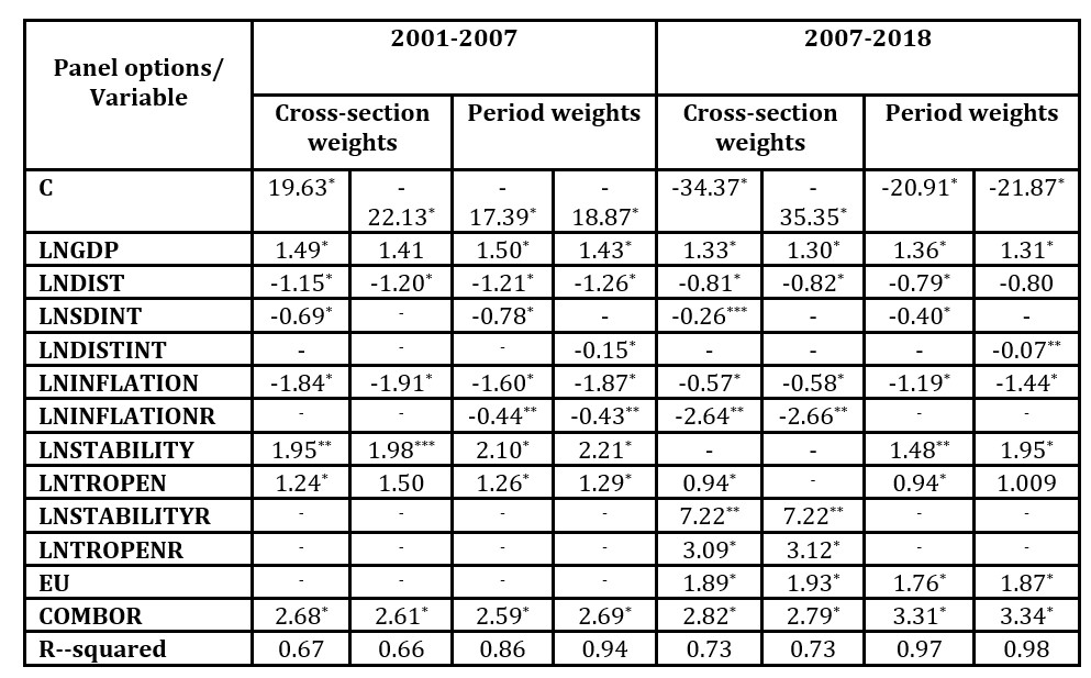
Table 2: The results for the panel regression before and after the EU integration

Legend statistically significant at 1% ^*, at 5% ^**, at 10%^***

Source: Author’s table based on the outputs

The same variables were tested for two periods: the one before 2007, which is the year of the Romanian integration in the EU and the period 2007-2018, when Romania has become an EU member.

In the pre EU period, some of the variables are not statistically significant: GDPR, STABILITYR, TROPENR and C in both versions and INFLATIONR in the first one. In the EU membership, the variables that are not statistically significant are: GDPR, STABILITYR in both versions, and DISTINT and C in the first one.

GDP explanatory power decreases from 1.7 before the EU integration to 1.3 after integration. The role of the distance between trading countries remains pretty much the same in the two considered periods, but the coefficients for the internal distances sharply increase after the EU integration.

The Romanian political stability and trade openness were not statistically significant before the EU integration, but became significant afterwards, while the trading partners’ stability was significant before the EU integration and not significant after it.

The trade openness of the partner countries becomes even more important after the EU integration and so the common border.

Two revised gravity equations are considered, removing the not statistically significant variables.

LNTRADE_t = c₀ + c₁LnGDP_t + c₂LnDIST + c₃LnSDINT + c₄LnINFLATION_t + c₅LnINFLATIONR_t + c₆ LnTRADEOPEN_t  + c₇LnSTABILITY_t + + c₈EU + c₉COMBOR + e_k

LNTRADE_t = c₀ + c₁LnGDP_t + c₂LnDIST + c₃LnDISTINT+ c₄LnINFLATION_t + c₅LnINFLATIONR_t + c₆ LnTRADEOPEN_t + c₇LnSTABILITY_t + c₈EU + c₉COMBOR + e_k

Table 3: The results for the panel second regression

Legend statistically significant at 1% ^*, at 5% ^**, at 10%^***

Source: Author’s table based on the outputs

For the period before the Romanian integration in the EU, these revised equations were considered:

LNTRADE_t = c₀ + c₁LnGDP_t + c₂LnDIST + c₃LnSDINT + c₄LnINFLATION_t + c₅LnINFLATIONR_t + c₆ LnTRADEOPEN_t  + c₇LnSTABILITY_t + + c₈EU + c₉COMBOR + e_k

LNTRADE_t = c₀ + c₁LnGDP_t + c₂LnDIST + c₃LnDISTINT+ c₄LnINFLATION_t + c₅LnINFLATIONR_t + c₆ LnTRADEOPEN_t + c₇LnSTABILITY_t + c₈EU + c₉COMBOR + e_k

Table 4: The results for the panel regression before and after the EU integration

Legend statistically significant at 1% ^*, at 5% ^**, at 10%^***

Source: Author’s table based on the outputs

Conclusions

The economic size of the partner countries positively influences the electronic trade flows. The coefficient for the Romanian GDP is negative, which is atypically; therefore, the first hypothesis is partially sustained. But how could this negative coefficient be explained? The deficit at the internal production, correlated with the internal demand, leads to relatively small Romanian exports and the Romanian economic growth is not significantly influenced by exports. By contrast, the imports had a sharp growth, which leads to a constant growth of the deficit of the trade balance. On the other side, the Romanian exports are based on low value, especially because of low wages compared to trading partners, so if the Romanian GDP would significantly grow, so would the wages and, therefore, the unit value for the exports, which would negatively influence the volume of the exports.

The second hypothesis is supported. In line with the previous studies, the distance between countries or the internal one has a negative impact on the electronics trade flows. The similar values for the sum of the internal distances and the distance between countries could be explained by the fact that a considerable share of the trade flows are with trading partners from Europe. The common border has a powerful positive impact on the electronics trade flows.

The membership in the same trade agreement and subquently the EU membership has a positive impact on the electronics flows, so the third hypothesis is supported.

The trading partners inflation negatively impacts the trade flows of a net electronics importer such as Romania, so the fourth hypothesis is sustained. As for the Romanian inflation, once more atypical results were found, namely negative, as well as positive coefficients. The consumer price index, which expresses the inflation, is based on a serie of statistic asimmetries because of mantaining the administrated prices, for instance on energy or natural gas. All these make the  dynamics of the exports and the dynamics of the inflation uncorrelated.

Trade policy factors, like trade openness, as well as political factors, like stability, positively impact the electronics trade flows, therefore, the last two hypothesis are fully supported.

References

• Abrams, R. K. (1980, March) ‘International Trade Flows under Flexible Exchange Rates’, Economic Review, Federal Reserve Bank of Kansas City, 3–10.
• Aitken, N. D. (1973) ‘The Effect of the EEC and EFTA on European Trade: A Temporal Cross-Section Analysis’, American Economic Review, 63, 881–892.
• Anderson, I. E. (1979) ‘A theoretical foundation of the gravity equation’, American Economic Review, 69 (1), 106-116.
• Anderson, J. E. (2011, September), ‘The Gravity model’, Annual Review of Economics, 3, 133-160.
• Anderson, J. E. and Neary, J. P. (2005)
  Measuring the Restrictiveness of International Trade Policy, MIT Press.
• Anderson, J. E. and van Wincoop, E. (2004) ‘Trade costs’, Journal of Economic Literature, 42, 691-751, DOI: 10.1257/0022051042177649.
• Anderson, J. E. and van Wincoop, E. (2003) ‘Gravity with gravitas: a solution to the border puzzle’, American Economic Review, 93 (1), 171-192, DOI: 10.1257/000282803321455214.
• Antonucci, D. and Manzocchi, S. (2006) ‘Does Turkey have a special trade relation with the EU? A gravity model approach’, Economic Systems, 30 (2), 157-169, DOI: 1016/j.ecosys.2005.10.003.
• Baier, S. L. and Bergsrtand, J. H. (2007) ‘Do free trade agreements actually increase members’ international trade?’, Journal of International Economics, 71 (1), 72-95.
• Baier, S. L. and Bergstrand, J. H. (2001) ‘The growth of world trade: tariffs, transport costs and income similarity’, Journal of International Economics, 53, 1-27, DOI: 10.1016/S0022-1996(00)00060-X.
• Baier, S. L. and Bergstrand, J. H. (2009) ‘Bonus vetus OLS: a simple method for approximating international trede-cost effects using the gravity equation’, Journal of International Economics, 77 (1), 77-85, DOI: 10.1016/j.jinteco.2008.10.004.
• Baier, S. L. and Bergstrand, J. H. (2004) ‘Economic determinants of free trade agreements’, Journal of International Economics, 64 (1), 29-63.
• Baier, S. L. and Bergstrand, J. H. (2009, February) ‘Estimating the effects of free trade agreements on international trade flows using matching econometrics’, Journal of International Economics, 77 (1), 63-76, DOI: 10.1016/j.jinteco.2008.09.006.
• Baldwin, R. and Taglioni, D. (2006) ‘Gravity for dummies and dummies for gravity equations’, NBER Working Paper N° 12516, (DOI): 10.3386/w12516.
• Baldwin, R. and Taglioni, D. (2011, January) ‘Gravity chains: Estimating bilateral trade flows when parts and components trade is important’, National Bureau of Economic Research (NBER). [Online], [Retrieved January 11, 2020], https://www.nber.org/papers/w16672.pdf .
• Baldwin, R. and Di Nino, V. (2006) ‘Euros and Zeros: The Common Currency Effect on Trade in New Goods’, NBER Working Paper W12673.
• Baltagi, B. H., Egger, P. and Pfaffermayr, M. (2003) ‘A generalized design for bilateral trade flow models’, Economics Letters, 80 (3), 391-397.
• Behar, A. and Nelson, B. D. (2014, July) ‘Trade Flows, Multilateral Resistance, and Firm Heterogeneity’, The Review of Economics and Statistics, MIT Press, 96 (3), 538-549.
• Bergrstrand, J. H. and Egger, P. (2009) Gravity Equations and Economic Frictions in the World Economy, Palgrave Handbook of International Trade, Bernhofen, D., Falvey, R., Greenaway, D. and Krieckemeier, U. (eds.), Palgrave-Macmillan Press, forthcoming.
• Bergstrand, J. H. (1990) ‘The Hecksher-Ohlin-Samuelson model, the linder hypothesis, and the determinants of bilateral intra-industry trade’, The Economic Journal, 100 (4), 1216-1229.
• Bergstrand, J. H. (1985) ‘The Gravity Equation in International Trade: Some Microeconomic Foundations and Empirical Evidence’, Review of Economic and Statistics, 67, 474–481.
• Bergstrand, J. H. (1989, February) ‘The Generalized Gravity Equation, Monopolistic Competition, and the Factor-Proportions Theory in International Trade’, Review of Economics and Statistics, 71 (1), 143-153.
• Blum, B. S. and Goldfarb, A. (2006) ‘Does the internet defy the law of gravity?’, Journal of International Economics, 70 (2), 384-405.
• Breuss, F. and Egger, P. (1999) ‘How reliable are the estimations of east-west trade potentials based on cross-section gravity analyses?’, Empirica, 26 (2), 81-94.
• Brun, J.-F., Carrère, C., Guillaumont, P. and de Melo, J. (2005) ‘Has distance died? Evidence from a panel gravity model’, The World Bank Economic Review, 19, 99-120.
• Bun, M. and Klaassen, F. (2002) ‘The importance of dynamics in panel gravity models of trade’, Tinbergen Institute Discussion Paper, No. 02–108/2.
• Burger, M. J., van Oort, F. G. and Linders, G. M. (2009) ‘On the specification of the gravity model of trade: zeros, excess zeros and zero-inflated estimation’, Spatial Economic Analysis, 4 (2), 167-190, https://doi.org/10.1080/17421770902834327.
• Cardamone, P. (2007) ‘A survey of the assessments of the effectiveness of Preferential Trade Agreements using gravity models’, International Economics, 60 (4), 421-473.
• Carrere, C. (2006) ‘Revisiting the effects of regional trade agreements on trade flows with proper specification of the gravity model’, European Economic Review, 50 (2), 223-247.
• Chaney, T. (2008) ‘Distorted gravity: the Intensive and extensive margins of International trade’, American Economic Review, 98, 1701-1721, DOI: 10.1257/aer.98.4.1707.
• Cheng, I.-H. and Wall, H. J. (1999, February) ‘Controlling for Heterogeneity in Gravity Models of Trade’, Working Paper, Federal Reserve Bank of St. Louis.
• Choi, C. (2002) ‘Linder hypothesis revisited’, Applied Economics Letters, 9 (9), 601–605, DOI: 10.1080/13504850110111234.
• Cipollina, M. and Salvatici, L. (2010) ‘Reciprocal trade agreements in gravity models: A Meta-Analysis’, Review of International Economics, 18, 63-80, https://doi.org/10.1111/j.1467-9396.2009.00877.x .
• Deardoff, A. (1998) Determinants of bilateral trade: does gravity work in a neoclassical world?, The regionalization of the world economy, Frankel, J. A. (ed.), Chicago, IL: University of Chicago Press.
• De Benedictis, L. and Taglioni, D. (2011) The Gravity Model in International Trade, The Trade Impact of European Union Preferential Policies: an analysis through gravity models, De Benedictis, L. and Salvataci, L. (eds.), Springer. Disdier AC.
• De Benedictis, L. and Vicarelli, C. (2005) ‘Trade potentials in gravity panel data models’, Topics in Economic Analysis & Policy, 5 (1), 1-31, DOI: 10.2139/ssrn.506562.
• De Benedictis, L. and Vicarelli, C. (2009) Dummies for gravity and gravity for policies: mission impossible?, Mimeo.
• Egger, P. and Pfaffermayr, M. (2003) ‘The proper panel econometrics specification of the gravity equation: a three-way model with bilateral interaction effects’, Empirical Economics, 28 (3), 571-580.
• Egger, P. (2002) ‘An econometric view on the estimation of gravity models and the calculation of trade potentials’, World Economics Journal, 25 (2), 297-312, https://doi.org/10.1111/1467-9701.00432 .
• Elliott, D.R., (2007) ‘Caribbean regionalism and the expectation of increased trade: insights from a time-series gravity model’, The Journal of International Trade & Economic Development, 16 (1), 117-136, https://doi.org/10.1080/09638190601165830 .
• Elmslie, B. (2018) ‘Retrospectives: Adam Smith’s Discovery of Trade Gravity’, Journal of Economic Perspectives, 32 (2), 209-222, DOI: 10.1257/jep.32.2.209.
• Evenett, S. J. and Keller, W. (2002) ‘On theories explaining the success of the gravity equation’, Journal of Political Economy, 110 (2), 281-316, DOI: 10.1086/338746.
• Fagiolo, G. (2010) ‘The international-trade network: gravity equations and topological properties’, The Journal of Economic Interaction and Coordination, 5, 1–25.
• Fajgelbaum, P. D., Grossman, G. M. and Helpman, E. (2011) ‘A Linder Hypothesis for Foreign Direct Investment’, NBER Working Papers 17550, National Bureau of Economic Research, Inc.
• Feenstra, R. C., Markusen, J. R. and Rose, A. K. (2001) ‘Using the gravity equation to differentiate among alternative theories of trade’, Canadian Journal of Economics, 34 (2), 430-447,https://doi.org/10.1111/0008-4085.00082 .
• Feenstra, R. C. (2002) ‘Border Effects and the Gravity Equation: Consistent Methods for Estimation’, Scottish Journal of Political Economy, 49 (5), 491-506, https://doi.org/10.1111/1467-9485.00244 .
• Fidrmuc, J. (2009) ‘Gravity models in integrated panels’, Empirical Economics, 37, 435-446.
• Filippini, C. and Molini, V. (2003) ‘The determinants of East Asian trade flows: a gravity equation approach’, Journal of Asian Economics, 14 (5), 695-711, DOI: 10.1016/j.asieco.2003.10.001.
• Gómez-Herrera, E. (2013) ‘Comparing alternative methods to estimate gravity models of bilateral trade’, Empirical Economics, 44 (3), 1087–1111.
• Grossman, G. (1996) Comments on Alan V. Deardorff. Determinants of bilateral trade: Does gravity work in a neoclassical world, The Regionalization of the World Economy, Frankel, J. A. (Ed.), University of Chicago for NBER, Chicago.
• Hallak, J. C. (2010, August) ‘A Product-Quality View of the Linder Hypothesis’, The Review of Economics and Statistics, MIT Press, 92 (3), 453-466.
• Haq, Z., Meilke, K. and Cranfield, J. (2010) ‘Does the Gravity Model Suffer from Selection Bias?’, Canadian Agricultural Trade Policy Research Network Working Paper no 90884, DOI: 10.22004/ag.econ.90884.
• Hatzigeorgiou, A. and Lodefalk, M. (2015, December) ‘Trade, Migration and Integration – Evidence and Policy Implications’, The World Economy, Wiley Blackwell, 38 (12), 2013-2048.
• Haveman, J. and Hummels, D. (2004) ‘Alternate Hypotheses and the Volume of Trade: The Gravity Equation and the Extent of Specialization’, Canadian Journal of Economics, 37, 199-218, https://doi.org/10.1111/j.0008-4085.2004.011_1.x .
• Head, K. (2008) ‘The puzzling persistence of the distance effect on bilateral trade’, The Review of Economics and Statistics, 90 (1), 37-48.
• Head, K. (2003) Gravity for beginners, Canada: University of British Columbia.
• Head, K. and Mayer, T. (2013) ‘Gravity Equations: Workhorse, Toolkit, and Cookbook’, Sciences Po Economics Discussion Papers, 2013-02, Sciences Po, Department of Economics.
• Helpman, E. and Krugman, P.R. (1985) Market Structure and Foreign Trade, Cambridge, Mass., MIT Press.
• Helpman, E., Melitz, M. and Rubinstein, Y. (2008) ‘Estimating trade flows: trading partners and trading volumes’, The Quaterly Journal of Economics, 123 (2), 441-487, https://doi.org/10.1162/qjec.2008.123.2.441 .
• Horsewood, N. (2009) ‘Are regional trading agreements beneficial? Static and dynamic panel gravity models’, The North American Journal of Economics and Finance, 20 (1), 46-65.
• Jung, W.-S., Wang, F. and Stanley, H. E. (2008) ‘Gravity model in the Korean highway’, Europhysics Letters, 81 (4), 1-13.
• Karemera, D., Koo, W., Smalls, G. and Whiteside, L. (2015) ‘Trade Creation and Diversion Effects and Exchange Rate Volatility in the Global Meat Trade’, Journal of Economic Integration, 30 (2), 240-268, DOI: 10.11130/jei.2015.30.2.240 .
• Keith, H. and Mayer, T. (2002) ‘Illusory Border Effects: Distance Mismeasurements Inflates Estimates of Home Bias in Trade’, Working Papers 2002-01, CEPII research centre, Paris.
• Keller, W. and Yeaple, S. R. (2009) ‘Gravity in the Weightless Economy’, NBER Working Paper No. 15509.
• Kimura, F. and Lee, H.-H. (2004, September 9-11) ‘The Gravity Equation in International Trade in Services’, European Trade Study Group Conference, University of Nottingham. [Online], [Retrieved January 9, 2020], http://cc.kangwon.ac.kr/~hhlee/paper/Kimura-Lee-040831.pdf .
• Krings, G., Calabrese, F., Ratti, C. and Blondel, V. D. (2009) ‘Urban gravity: a model for inter-city telecommunication flows’, Journal of Statistical Mechanics, https://iopscience.iop.org/article/10.1088/1742-5468/2009/07/L07003/pdf.
• Lawless, M. (2010) ‘Deconstructing gravity: trade costs and extensive and intensive margins’, Canadian Journal of Economics, 43 (4), 1149-1172, https://doi.org/10.1111/j.1540-5982.2010.01609.x .
• Levine, R. and Renelt, D. (1992) ‘A Sensitivity Analysis of Cross-Country Growth Regressions’, American Economic Review, 82 (4), 942-963.
• Linder, S. B. (1961) An Essay on Trade and Transformation, New York: John Wiley and Sons.
• Linders, G. J. and de Groot, H. L. F. (2006) ‘Estimation of the Gravity Equation in the Presence of Zero Flows’, Tinbergen Institute Discussion Paper No. 06-072/3.
• Lorde, T., Li, G. and Airey, D. (2015) ‘Modeling Caribbean tourism demand: an augmented gravity approach’, Journal of Travel Research, 1-11, https://doi.org/10.1177/0047287515592852 .
• Magerman, G., Studnicka, Z. and Van Hove, J. (2016) ‘Distance and Border Effects inInternational Trade: A Comparison of Estimation Methods’, Economics E-Journal, 10 (18), 1-31, http://dx.doi.org/10.5018/economics-ejournal.ja.2016-18 .

• Martin, W. and Pham, S. C. (2008) ‘Estimating the Gravity Equation when Zero Trade Flows Are Frequent’, World Bank.
• Martinez-Zarzoso, I. (2013), “The log of Gravity Revisited”, Applied Economics, 45 (3), 311-327.
• Martínez-Zarzoso, I. and Nowak-Lehman, F. (2003) ‘Augmented Gravity Model: An Empirical Application to Mercosur-European Union Trade Flows’, Journal of Applied Economics, 6, 291-316.
• Masucci, A. P., Serras, , Johansson, A. and Batty, M. (2013) ‘Gravity versus radiation models: On the importance of scale and heterogeneity in commuting flows’, Physical Review E., 88 (2): 022812, https://doi.org/10.1103/PhysRevE.88.022812 .
• Melitz, J. (2007) ‘North, South and distance in the gravity model’, European Economic Review, 51 (4), 971-991, DOI: 10.1016/j.euroecorev.2006.07.001.
• Miron, D., Cojocariu, R. C. and Tamaș, A. (2019) ‘Using Gravity Model to Analyze Romanian Trade Flows between 2001 and 2015’, Economic Computation and Economic Cybernetics Studies and Research, 53 (2), 5-22, DOI: 24818/18423264/53.2.19.01.
• Papazoglou, C. (2007) ‘Greece’s potential trade flows: a gravity model approach’, International Advances in Economic Research, 13 (4), 403-414, DOI: 10.1007/s11294-007-9107-x.
• Pollins, B. M. (1989) ‘Conflict, Cooperation, and Commerce: The Effect of International Political Interactions on Bilateral Trade Flows’, American Journal of Political Science, 33 (3), 737-761, DOI: 10.2307/2111070.
• Porojan, A. (2001) ‘Trade flows and spatial effects: the gravity model revisited’, Open Economies Review, 12, 265-280.
• Portes, R. and Rey, H. (2005) ‘The determinants of cross-border equity flows’, Journal of International Economics, 65 (2), 269-296, doi:10.1016/j.jinteco.2004.05.002.
• Pöyhönen, P. (1963) ‘A Tentative Model for the Volume of Trade Between Countries’, Weltwirtchaftliches Archiv, 90, 93-100.
• Roberts, B. A. (2004) ‘A gravity study of the proposed China-Asean free trade area’, The International Trade Journal, 18 (4), 335-353, https://doi.org/10.1080/08853900490518208 .
• Sanso, M., Rogelio, C. and Sanz, F. (1993) ‘Bilateral Trade Flows, the Gravity Equation, and Functional Form’, The Review of Economics and Statistics, 75, 266–275.
• Santos Silva, J. M. C. and Tenreyro, S. (2006) ‘The log of gravity’, The Review of Economics and Statistics, 88 (4), 641-658.
• Santos Silva, J. M. C. and Tenreyro, S. (2009) ‘Trading Partners and Trading Volumes: Implementing the Helpman-Melitz-Rubinstein Model Empirically’, CEP Discussion Paper No 935.
• Santos Silva, J. M C. and Tenreyro, S. (2011) ‘Further Simulation Evidence on the Performance of the Poisson-PML Estimator’, Economics Letters, 112 (2), 220–222.
• Shepherd, B. (2008) ‘Behind the Border- Gravity Modelling’, Asia-Pacific Research and Training Network on Trade (ARTNeT), Capacity Building Workshop (December 14-19, 2008), Bangkok, Thailand.
• Siliverstovs, B. and Schumacher, D. (2008) ‘Estimating gravity equations: to log or not to log?’, Empirical Economics, 36 (3), 645-669, DOI 10.1007/s00181-008-0217-y.
• Söderström, J. (2008) Cultural Distance An Assessment of Cultural Effects on Trade Flows, Master Thesis.
• Sohn, C.-H. (2005) ‘Does the gravity model explain South Korea’s trade flows?’, The Japanese Economic Review, 56 (4), 417-430, DOI: 10.1111/j.1468-5876.2005.00338.x.
• Stavytskyy, A., Kharlamova, G., Giedraitis, V. and Sengul, E. C. (2019) ‘Gravity model analysis of globalization process in transition economies’, Journal of International Studies, 12 (2), 322-341, doi: 10.14254/2071-8330.2019/12-2/21.
• Stockman, A. C. (1981) ‘Anticipated inflation and the capital stock in a cash in-advance economy’, Journal of Monetary Economics, 8 (3), 387-393.
• Tamaș, A. (2019) ‘An Augmented Gravity Model Using Linder Variable to Study UK Tourism Flows’ Proceedings of the 33 International Business Information Management Association Conference (IBIMA): Education Excellence and Innovation Management through Vision 2020, ISBN: 978-0-9998551-2-6, 10-11 April 2019, Granada, Spain, 215-226.
• Tamaș, A. (2017) ‘Romanian Erasmus Students’ Flows – Gravity Model Approach’, Journal of Eastern Europe Research in Business and Economics, 2017 (2017), 1-11, DOI: 10.5171/2017.253964.
• Tamaș, A. (2017) ‘The Design of the Romanian Wine Imports and Exports Using the Gravity Model Approach’, International Journal of Business and Management, V (2), 64-77, DOI:20472/BM.2017.5.2.005.
• Timbergen, J. (1962) Shaping the World Economy: Suggestions for an International Economic Policy, New York: The Twentieth Century Fund, https://doi.org/10.2307/1236502 .
• Thursby, J. G. and Thursby, M. C. (1987) ‘Bilateral Trade Flows, the Linder Hypothesis, and Exchange Risk’, Review of Economics and Statistics, 69 (3), 488-495, DOI: 10.2307/1925537.
• Tzouvelekas V. (2007) ‘Accounting for pairwise heterogeneity in bilateral trade flows: a stochastic varying coefficient gravity model’, Applied Economics Letters, 14 (12), 927-930, DOI: 10.1080/13504850600705919.
• Westerlund, J. and Wilhelmsson, F. (2009) ‘Estimating the Gravity Model without Gravity using Panel Data’, Applied Economics, 41, 1-9, DOI: 10.1080/00036840802599784.

www.cepii.fr › pdf_pub 

www.chemical-ecology.net

https://data.worldbank.org ›

https://www.theglobaleconomy.com › rankings