This paper tests the profitability of momentum strategies in Kenya, an emerging market for the period 1995 to 2007. Both relative strength strategies (RSS) and (weighted relative strength strategies (WRSS) are employed to implement momentum-based trading strategies. Analysis revealed that Nairobi Stock Exchange (NSE) exhibit medium term return continuation over the entire sample period and the sub-periods. We used RSS results to evaluate the influence of transaction costs, calendar effects, risk factors and other reported momentum characteristics on momentum profitability. We employ WRSS results to discriminate between the two diametrically opposed causes for the profitability of momentum strategies: behavioral factors (time-series continuation in the firm-specific component of returns), and risk factors (cross-sectional variation in expected returns and systematic risks of individual securities). Our results show that, consistent with the evidence elsewhere, momentum is an anomaly; the evidence is consistent with momentum being driven by continuation in the idiosyncratic component of individual-security, rather than by cross-sectional differences in expected return and risks.
The concept of Efficient Market Hypothesis (EMH) appeared in 1960s and reached such a height of dominance around 1970s that any deviation in financial markets has been called anomaly. The 1980s witnessed the proliferation of reported anomalies. Among them, medium-term continuation of equity returns, also called “momentum strategy”, is the most intriguing phenomenon. It has not been traded away, despite being well known as public information for many years now.
Jegadeesh and Titman (1993, 1995) are the first to report medium-term profit “momentum”. Upon examining a variety of momentum strategies in the United States stock market over the sample period 1965 to 1989, they find that strategies that buy winning stocks (stocks with high returns over the previous three months to one year) and sell losing stocks (stocks with low returns over the same period) earn profits of about 1 percent per month for the following year.
Since its very first appearance as an anomaly to the EMH, momentum has been criticized by many as the product of a data snooping process. But out of sample testing has vindicated the widespread existence of the momentum phenomenon. Jegadeesh and Titman (2001) extend the original sample period to the period of 1990 to 1998, and confirmed the same level of profits reported in their seminal paper. Grundy and Martin (2001) further extend the sample period and document that momentum profits are remarkably stable across sub-periods post 1926.
Besides, other researchers have checked stock markets of different regions over different time periods using various methods, and have consistently reported positive returns by implementing these strategies. Rouwenhorst (1998) for instance, documents momentum profits for several European markets, of similar magnitude to those in the USA. In the Asian markets, Chui et al. (2000) reports evidence of momentum profitability. There is evidence that investors employ momentum strategies in making decisions. Grinblatt et al. (1995) report that, about 77% of the investors in their sample, have recourse to momentum strategizing.
The proponents of EMH argue that the momentum results can be accounted within the framework of risk factor models. Zarowin (1990) attributes them to the size factor effect: Small stocks, often losers, have higher expected return than large stocks. Chan et al. (1996) show that medium-term performance continuation can be partly explained by underreaction to earnings information, but price momentum is not subsumed by earnings momentum. Fama and French (1996) try to account for the cross-section stock return predictability with their multifactor model, but fail to explain medium-term return continuation. Chopra et al. (1992) show that losers would have to have much higher betas than winners in order to justify the return differences, and the beta in the CAPM framework cannot account for it. Grundy and Martin (2001) find that neither industry effects nor cross-sectional differences in expected returns are the primary cause of the momentum phenomenon, and the strategy’s average profitability cannot be explained by Fama and French’s three-factor model.
Some behavioral models have been suggested to explain the momentum strategy. Grinblatt and Han (2001) argue that the disposition effect accounts for a large percentage of the momentum in stock returns. The concavity (convexity) of the value function in the gains (losses) region makes investors willing to sell (hold) a stock which has earned them capital gains (losses). And this may initially depress (inflate) the stock price, generating higher (lower) returns later. Hirshleifer and Shumway (2003) attribute the momentum to the fact that low returns on a stock put the investors of the stock in a negative, critical mood. This bad mood may in turn cause skeptical and pessimistic interpretation of subsequently arriving information. People will not fully foresee their negative interpretation of future information, causing a tendency toward continuation of the drop in price. Other behavioral models include Barberis et al. (1998), Daniel et al. (1998), and Hong and Stein (1999).
In his response to the critiques of the EMH, Fama (1998) argues that the return anomalies should stand up to out-of-sample tests. If the conclusions derived from developed markets are robust, we should find similar effects in developing markets. Since Kenyan market can be considered to be independent of the developed world, findings of a momentum pattern in Kenya should contribute evidence that puts to rest the fears of data snooping.
The objectives of the study are four-fold. Firstly, we test the pervasiveness of profitability of momentum strategies using data from the NSE. Secondly, we check whether transaction costs and risk factors can significantly dissipate momentum profits when taken into account. Thirdly, we examine whether the characteristics of momentum profits reported in the literature, such as calendar effect, apply to the NSE. And fourthly, we decompose the momentum profits, using the framework of Conrad and Kaul (1998) and evaluate the relative importance of the behavioural component (time series predictability) versus the risk-based component (cross-sectional variation).
We find that “Winners” outperform “Losers” in the medium-term horizons for nearly all holding periods. The outperformance lasts for about one and half years. Further tests show that the momentum returns cannot be explained by the Fama-French three-factor model. Different from developed markets (USA), we do not observe the January effect at the NSE. Furthermore, transaction costs do not rule out the profitability of the momentum strategies for a majority of the holding periods. Contrary to Conrad and Kaul (1998) who report a negligible role of the time-series predictable components in the United States market, we find that the expected profits are highly predictable for most of the trading strategies from the time-series. Besides, the cross-sectional variance of mean returns of individual securities increases with the trading horizon, but the magnitude of the increase is much smaller than the random walk hypothesis predicts.
Nairobi Stock Exchange (NSE)
Daily prices of stocks listed at the NSE obtained covering the period 1995 to 2007. The prices were used to derive average monthly prices which were adjusted for stock splits and bonus issues. With these data, we calculate profits of various momentum strategies from January 1996 to December 2007. The data for 1995 were mainly used in constructing the beginning relative strength portfolios. Part of our tests employed Fama and French three-factor model, it was necessary to collect data on relevant variables. We used the NSE_20 index as proxy for the market. To calculate excess market return, the risk free rate of return will be estimated from The Government Treasury Bill rate which is obtained from the Central Bank of Kenya.
The trends, once noting in Table 1, are for the averages of the market return and the risk-free rate. The return on the NSE 20 index (proxy for the market portfolio) averages approximately 0.05% for the whole sample period. The sub-period 1997-2002 was characterized by a decline in the index, with markets monthly returns registering -1.04%. In contrast, the sub-period that followed between the years 2003 to 2007, coincided with and exuberant mood among investors with the consequence that monthly market returns averaged 2.42%.
The risk-free rate experiences opposite trends to the market return. For the sub-period 1997-2002, the Treasury bill rate spiked up, registering a monthly average return of 1.29%. In this period the government of the day raised the interest on treasury bills so as to attract domestic finance to bridge a gap left by international donors who reneged on the aid pledges. The sub-period 2003-2007 sees a drastic fall in the average monthly risk-free rate to 0.057%, reflecting a phase of prudent financial management and the unlocking of donor funds, mainly because of the change in political power dispensation at the end of 2002.
Table 1 also reports the SMB and HML factors of Fama-French for the sample markets. To calculate these factor values, we follow the method described in Fama and French (1993) to form the 6 size-BE/ME stock portfolios based on all the equities at the Nairobi Stock Exchange.
Table 1: Descriptive Statistics of Equities in the Sample and Sub-samples
* This table gives the monthly descriptive statistics of the Nse20 index (a proxy for the market), and the Fama-French factors for the Nairobi stock Exchange for the whole sample period and sub-samples. To calculate these values the method of Fama and French (1993) was followed by forming 6 size-BME stock portfolios based on all equities listed.
Data Analysis, Findings and Discussions
Profits of Relative Strength Strategy (RSS)
First, we form the relative strength portfolios as described in Jegadeesh and Titman (1993). At the end of each month t, all stocks are ranked in descending order on the basis of their past J months’ returns (J = 3, 6, 9, or 12). Based on these rankings, the stocks are assigned to one of five quintile portfolios. The top quintile portfolio is called the “Winner”, while the bottom quintile called the “Loser”. These portfolios are equally weighted at formation, and held for K subsequent months (K=3, 6, 9, and 12). See Appendix I in appendices.
To understand the notion of strategic human resource management, it is necessary to appreciate the concept of strategy upon which it is based. Johnson and Scholes (1999) define strategy as the direction and scope of an organization over the long term which achieves advantage for the organization through configuration of resources within a changing environment, to meet the needs of markets and fulfill shareholders expectations.
Mintzberg et al (1988) suggest that strategy can have a number of meanings namely; a plan or something equivalent- a direction; a guide or cause of action; a pattern that is consistency in behavior over time; a perspective, an organizations way of doing things; a play, a specific maneuver intended to outwit an opponent or a competitor.
Pearce and Robinson (2000) recommend three critical ingredients for the success of a strategy. First, the strategy must be consistent with conditions in the competitive environment. It must take advantage of existing or projected opportunities and minimize the impact of major threats. Second, the strategy must place realistic requirements on the firm’s resources. The firm’s pursuit of market opportunities must be based not only on the existence of external opportunities but also on competitive advantages that arise from the firm’s key resources. Finally, the strategy must be carefully executed.
To minimize small-sample biases and to increase the power of the test, we implement trading strategies for overlapping holding periods on a monthly frequency. Therefore, in any given month t, the strategies hold a series of portfolios that are selected in the current month as well as in the previous K-1 months. This is equivalent to a composite portfolio in which 1/K of the holding is replaced each month. To avoid the potential “survival biases”, we do not require all securities included in a particular strategy in the formation period to survive up to the end of the holding period. If a security i survives for less than J periods, we use a (J-j) period in calculating returns, where j is the period of delisting. If a security does not survive the formation period, it is dropped from the particular strategy.
Appendix I shows the average monthly buy-and-hold returns on the composite portfolio strategies implemented during different periods at the NSE. For each strategy, the table lists the returns of the “Winner” and the “Loser”, as well as the excess returns (and t -stat) from buying “Winner” and selling “Loser”. For instance, as Panel A shows, during the period 1996-2007 buying “Winner” from a 3-month/3-month strategy earns an average return of 1.31 percent per month, 0.85 percent higher than buying “Loser” in the same strategy, which returns 0.46 percent. The excess return is significant at the 5 percent level of significance, with a t -stat of 1.714
For the entire period 1996-2007, among the sixteen strategies implemented, significantly positive excess returns are observed at the 5 percent level for nine strategies. Specifically, the excess returns of buying “Winner” over buying “Loser” range from -0.28 for the 3-by-12 strategy to 1.72 percent per month for the 9-by-9 strategy (with a mean of 0.54 percent).
The portfolio returns of both sub-periods are in stark contrast. The sub-period 1996 to 2002 is characterized by a complete lack of momentum in the returns. Of the 16 strategies implemented over the period, only four show significant momentum profitability. Of the remaining portfolios, significantly negative returns are experienced for 8 strategies. The average Winner-Loser return for the period is virtually zero percent (0.019 percent).
The period 2003 to 2007 is responsible in large measure for the momentum effect witnessed in our overall sample. Fifteen of the strategies during this period exhibit positive momentum profits that are significant at the 1% level. Average monthly momentum profits are at 1.23 percent, and ranging between–0.16 percent to 3.5 percent per month.
We include the sub-periods to investigate the robustness of the momentum at the NSE. The evidence from our analysis is mixed. While in one period, momentum is not discernible, a later period provides unmistakable evidence of the continuation phenomenon. In sum, the balance of evidence dips on the side existence of momentum effect.
Characteristics of Momentum Strategies (with RSS)
Risk-Adjusted Returns
This subsection explores the relationship between the returns of momentum portfolios and Fama-French risk factors, namely, the overall market factor (the value-weighted NSE20 index minus the risk-free rate), the size factor (SMB, small stocks minus big stocks), and the book-to-market factor (HML, high minus low book-to-market stocks). We regress the monthly returns of the momentum strategy in excess of the risk-free interest rate, on the excess return of the NSE20 index over the risk-free interest rate, and the Fama-French SMB and HML factors over thesample periods. The regression takes the form below:
(4.1)
Where
=Average return of the relative strength strategy for the month t. The risk free rate of return observed at the beginning of the month, t.
Average monthly return on the overall market factor The monthly difference between the returns of a portfolio of small stocks and the portfolio of big stocks
The monthly difference between the returns of a portfolio of high BE/ME stocks and the portfolio of low BE/ME stocks
The intercept in the regression equation
The sensitivity of the size factor to relative strength strategy (RSS) profits
The sensitivity of RSS profits to the overall market factor
The sensitivity of RSS profits to the B-M factor
The error term of the regression
Table 2: Risk Adjusted Excess Returns of Momentum Portfolios
* This table provides the results from regression the monthly returns of the 6-month/6-month momentum strategy in excess of the risk-free interest rate on Fama-French three-factors:
over the sample period:
is the coefficient of determination adjusted for degrees of freedom;is the related coefficient divided by its standard error.
**significant at 1%: * significant at 5%.
Table 2 reports the results of the regression for the whole period and the two sub-periods. As is shown in column 4, all the market factor coefficients are negative, indicating that the losers are somewhat more sensitive to the market risk factor than the winners. A closer look at column 5 shows that coefficients for the whole sample and 1996-2002 sub-period are significantly different from zero, meaning that market betas forwinners and losers differ significantly. Columns 6-9 reveal the effect of the size factor coefficients and book-to-market factor coefficients . The signs are mostly negative and the significant levels are mixed.
This indicates that the losers are riskier than the winners because they are relatively more sensitive to all three Fama-French factors.
The second column of Table 2 reports the alpha (α) of the various momentum portfolios estimated by regressing the monthly momentum returns on the Fama-French factors. The alphas for these risk-adjusted portfolios are about the same as the raw returns, with the only exception of the 1997-2002 sub-period which registers alpha significantly equal to zero.
The last column of the table presents the R-square of each regression, ranging from 0.082 to 0.0.627. In sum, the Fama-French three-factor model cannot explain the profits of the momentum strategies in most of the cases.
Seasonality Effect
Jegadeesh and Titman (1993, 2001) find an interesting seasonality in momentum profits in the United States. They document that the Winners outperform the Losers in all months except January, when the Losers outperform the Winners. Grundy and Martin (2001) also report similar results in the U.S., where the momentum portfolio earns significantly negative returns in Januaries and significantly positive returns in months other than January. Might this seasonality be a statistical fluke? We examined the performance of the strategy in January and non-January months to see whether the January effect applies at NSE. Table 3 reports the average monthly momentum portfolio returns and the percentage of months with positive returns for January as well as non-January months. Column 3 in the table is the associated t-statistics. Different from earlier findings in the United States market, the momentum profits in January at NSE show significant positive returns. This result is consistent with the findings of Wang (2008) on the markets of UK, Germany, Japan, and China.
Table 3: Momentum Returns in January and Outside January
* This table reports the average monthly momentum portfolio returns, associated t-statistic, and the percentage of positive returns for January as well as non-January months. The momentum portfolios are formed based on previous six-month returns and held for six months. The table also reports the difference between the January monthly returns and the non-January monthly returns.
**Significant at 5% level. *** Significant at 1% level.
Table 3 also reports the test of the difference between the average monthly January returns and the average monthly non-January returns. Not surprisingly, the difference is insignificant.
Post-holding Period Cumulative Profits to the Momentum Strategy
In this subsection we examine the results of momentum portfolios over various holding time horizons (K) to check the behavior of the momentum returns over time. This provides information on the duration of the continuation effect and the extent to which it is permanent. Table 4 gives the monthly average momentum portfolio returns and associated t-statistics in the first five years after portfolio formation based on previous six-month returns. The returns are nearly positive in the first year, after which they turn negative. These results are very similar to Jegadeesh and Titman (1993) for the United States, who report dissipation and reversal of momentum profits after one year, in the United States.
Table 4: Post-holding Period Returns
* This table reports the average monthly momentum portfolio returns and associated t-statistic over a 60-month post-formation period… The momentum portfolios are formed based on previous six-month returns. The number in bold means significantly, different from zero at 5% level. Compared to other markets, momentum at the Nairobi stock exchanged is apparently a very short-lived phenomenon, lasting only for only 8 months. Starting from the 9th holding month, momentum persists but not at a significant magnitude. By the 24th month momentum has petered out and mild reversal is observed up to the 60th holding month.
Appendix II depicts the evolution of the cumulative momentum profits over an event time of 60-month post-formation period. Cumulative momentum profits increase monotonically in the first two years until they reach the peaks between 10 and 20 percent. The NSE shows a degree of reversal but maintains a profit level of above 5%. These results are consistent with the behavioral models that predict that momentum profits will be reversed eventually. See appendix II,Cumulative Momentum Profits.
This figure presents cumulative momentum portfolio returns of RSS over a 60-month post formation period. The sample stocks cover over 95 percent of the market capitalization in each country. The momentum portfolios are formed based on previous six-month returns.
Transaction Costs
Transaction costs of implementing the momentum strategies may cancel out all or part of the momentum profits documented.
Transaction costs for a single transaction at the NSE amount to 2 % in form of brokerage commissions and various fees and levies paid to the stock exchange and related regulatory agencies This implies roundtrip transaction cost of 4 per cent. Assuming a transaction frequency of 40 percent1, this cost per transaction is reduced to 1.6 % per transaction. For momentum trading to earn abnormal profits, it must return a rate significantly higher than 1.6 percent. Does our 6 month/ 6 month strategy meet this minimum condition?
1Grundy and Martin (2001) report an average 40 percent of turnover for both the winner and the loser portfolios
The 6 month / 6 month strategy requires four trades per six month period (opening and closing positions for both the Winner and loser portfolios. Our strategy reported earlier in Appendix I, results in six-month average return of 7.02%. With a requirement of four transactions to close the position, this delivers a return of 1.8 percent per transaction. This return compares unfavourable with transaction costs of 1.6 percent. Even if one revises the adapted trading frequency which should lower for illiquid markets like the NSE, the level of comfort for these strategies is still marginal. This is because, while this simple approximation accounts for the dynamics of the trading strategy by incorporating the transaction costs when they occur, it neither considers market frictions induced by trading (i.e., a price impact) nor attempts to account for potential differences in trading costs associated with different stocks or stock characteristics. For simplicity, we just assume that transaction costs for buying and selling winner stocks as well as selling short and buying back loser stocks are of equal size. Lesmond et al. (2004) have indeed shown that many of the stocks included in relative strength strategies are illiquid and extreme, and require disproportionately high levels of transaction costs to trade.
Whether momentum strategies are anomalous, may ultimately depend on the answers surrounding the costs of trading the strategies. It appears evident that transaction costs when properly modelled and incorporated in the analysis have the potential to eat away into any illusory abnormal profits. The efficient markets hypothesis that has been retreating in the face of the relentless march of behavioural scientist may find here saving grace and be eventually vindicated as the foundation of asset pricing.
From the analysis, we conclude that momentum strategies remain highly profitable also when transaction costs are accounted for. Though we acknowledge that the preceding analysis provides only a crude approximation to the effect of transaction costs on the profitability of our momentum strategies, it is patent that momentum strategies may be very profitable, at least not to the degree touted by proponents.
Nevertheless, as shown by Appendix II, the absolute value of cumulative momentum profits significantly exceeds a 1.6 percent transaction cost for holding periods between 12 and 36 months. It appears plausible that long horizon holding periods which need less frequent trading can be profitable. This notion underlies the results of Wang (2008) finding for four markets: that the momentum profits obtained in each market remain significantly different from zero after considering the transaction costs.
Decomposition of the Profit Sources (with WRSS)
To enable us decompose momentum profits we generate them using the weighted relative strength method of Conrad and Kaul (1998)2 .
2 Jegadeesh and Titman (1993) report a correlation as high as 0.95 for the 6-month/6-month strategy in the United States. Wang (2008) reveals, in his study of UK, Germany, Japan, and China markets, that the e returns of RSS and WRSS are evidently positively correlated.
As in the section under relative strength strategies, the test period is divided into J-month formation period (from time t-2 to t-1) and k-month holding period (from time t-1 to t). Following Conrad and Kaul (1998), the weight of each security in the trading portfolio in the holding period is determined by the relative performance of the security to the equal-weighted market portfolio in the formation period. Specifically, (4.2)3
3 The plus sign in the equation emphasizes that we will implement a moment strategy, i.e., going long in a security if it outperforms the equal-weighted market portfolio and going short in a security if it underperforms the market portfolio.
where is the fraction of the trading strategy portfolio devoted to security i, in holding period, is the return of security i in the formation period, and is the equal-weighted market portfolio return in the formation period. N is the number of securities in the portfolio at time t-1, and i=1… N.
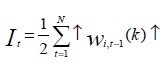
By construction, the portfolio is an arbitrage portfolio since the weights of securities sum to zero. And the total investment position (long or short) is given by:
(4.3)
The profit in the holding period for the strategy is:
(4.4)
For the 6-by-6 strategy the results of the WRSS strategy range from -0.012 to0.019, with a mean of 0.012. The correlation between the RSS results and the WRSS results is high at 0.845.
After generating the WRSS returns, we next decompose the profits of weighted relative strength strategies (WRSS) and investigate the source of the momentum profits. To decompose the WRSS profit, we assume that the realized return of stock i is expressed as:
(4.5)
where is the unconditional expected return of stock i and is the unexpected return at time t. Then the
momentum profits in Eq. (4.5) can be decomposed into components based on expected and unexpected components of returns as follows:
(4.6)
Where is the first-order auto-covariance of the returns on the market portfolio, is the average of the first-order auto-covariances of the N individual stocks in the zero cost portfolio, , and is the cross-sectional variance of expected returns4 . In calculating the components of the trading portfolio profits, we assume that individual stock returns are mean stationary.
4 Lo and MacKinlay (1990) originally propose this decomposition. Jegadeesh and Titman(1995), and Conrad and Kaul (1998) have further treatment of this decomposition and its economic interpretation.
Eq. (4.6) decomposes the total expected profits into two components:P(K) ; the time-series predictable components in asset returns, and ; the profits generated by cross-sectional variance of the mean returns. The equation indicates that any cross-sectional variation in expected returns contributes positively to momentum profits. Since realized past returns are positively correlated with expected returns, if a large part of realized returns is due to expected returns, past Winners (Losers) will, on average, continue to earn higher (lower) than average returns in the future.
Following Conrad and Kaul (1998), we assume that the serial covariances and the cross-sectional variances of mean returns of individual stocks are time dependent.
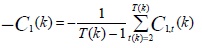
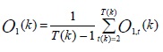
Then, , and are estimated as:
(4.7) Where
(4.8) Where
And
(4.9) Where
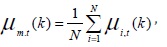
T (k) is the total number of overlapping returns in the sample period for a trading strategy of holding period , are the estimated expected returns of stock i , and market portfolio at time t-1. is estimated through average realized returns of each stock:
(4.10)
Where
is the number of observations available for stock i . Then, (4.11)
Table 5 presents the results of the contribution of time-series predictability and cross-sectional variation of stock returns over different holdings k for the entire sample period, where k ranges from 3 to 12 months. For brevity, we only list strategies for which the length of the formation period J and the future holding period k are identical. Their results are representative for other strategies with different formation and holding periods.
The columns 2-4 report, , P(k), and . To facilitate evaluation of the relative importance of the profit sources, the percentage contributions of P(k), and to the total profits, , are reported in column 5 and column 6, respectively.
There are several notable findings in Table 5. First, is significant in all cases, given the fact that is the cross-sectional variance of .
The P(k) is negative but insignificantly different from zero. Second, the magnitude of P(k) increases monotonically with time. The percentage contribution of P(k) dominates that of in nearly all strategies.
Table 5: The Decomposition of Average Profits to WRSS
*This table reports the decomposition of average profits to trading strategies and associated t-statistics (with identical formation and holding period during its entire sample period. The decomposition is given by , where P(k) and represent the time-series and cross-sectional predictable parts, respectively. All profit estimates are multiplied by 100. * and † denote significance at 5% and 10%, respectively.
The results are revealing in two ways. First, the expected profits are highly predictable for most of the trading strategies from the time-series components, since P(k) contributes more of the profits than does. This finding is different from the United States market results by Conrad and Kaul (1998). Second, the results do not support the random walk hypothesis.
Although the magnitude of does increase with the trading horizon, the magnitude of the increase is much smaller than the random walk hypothesis indicates. In sum, these results reveal market inefficiencies.
Conclusions
This paper documents returns of momentum strategies at the NSE during the period 1997 to 2007. Following the framework developed by Jegadeesh and Titman (1993) and Conrad and Kaul (1998), we measure the momentum profits of WRSS. It turns out that the past Winners outperformed the past Losers for most of the periods. Further tests show that the momentum returns cannot be explained by risk models such as the Fama-French three-factor model. Different from the United States market, we do not observe the January effect in our sample markets. The concavity of the cumulative momentum profits over various holding periods show that the behavioral models are supported. When trading, costs are considered, however, relative strength strategies’ profitability is significantly vitiated especially for a majority of short horizon holding periods of over 12 months. We decompose the expected profits of the momentum strategies into two different sources: Time-series profitable component and cross-sectional variance of mean returns of individual securities. We find that the expected profits are highly predictable for most of the trading strategies from the time-series components. In addition, the cross-sectional variance of mean returns of individual securities increases with the trading horizon, but the magnitude of the increase is much smaller than the random walk hypothesis predicts. These results cast doubts on market efficiencies.
Chui, A., Titman, S. & Wei, K. (2000). “Momentum, Ownership Structure, and Financial Crises: An Analysis of Asian Stock Markets,” University of Texas at Austin Working Paper. Google Scholar
Appendix I: Average Profits to Relative Strength Strategies (RSSs)
*The table shows average profits to relative strength strategies (RSS) at the NSE between 1995 to 2007, and two sub-periods to distinguish a markedly bullish posr-2002 period from the earlier period. At the end of each month t, all stocks at the stock marked are ranked in descending order on the basis of their J-months’ past returns. Based n these rankings the stocked are assigned to each of the equally weighted 5 quintile portfolios. The top quintile portfolio is called the “Winner”, while the bottom quintile portfolio is called the “Loser”. These equally weighted portfolios are held for K subsequent months. t-statistic is the average return divided by its standard error.* represents significance at the 5% level and ** significant at 1% level