Bucharest Academy of Economic Studies, Bucharest, Romania
Volume 2021,
Article ID 726877,
Journal of Financial Studies and Research,
28 pages,
DOI: 10.5171/2021.726877
Received date: 5 September 2019; Accepted date: 11 July 2021; Published date: 13 October 2021
Cite this Article as:
Andreea OPREA (2021)," On the Assessment of the V-Inverted Shape Pattern for Romanian Government Bond Yields Around Treasury Auctions", Journal of Financial Studies & Research, Vol. 2021 (2021), Article ID 726877, DOI: 10.5171/2021.726877
In this paper, we intend to provide some theoretical and practical insights on the interdependence between treasury auctions and market yields around auction time. Based on previous research, we investigated the presence of the auction cycle and the corresponding V-inversed pattern of yields in the case of the Romanian sovereign bond market. For the 2-, 4- and 5-year on-the-run government bonds we found statistical evidence that a V-inversed pattern or a partial pattern emerged around auction days.This evidence supports the theory that primary dealers tend to liquidate positions prior to treasury auctions so that they can take on more risk. Apart from the auction cycle which based on the Romanian bond market specificities was considered to be of length 5 (composing the auction day and 2 days prior and after the auction), we also investigated the intraday behavior of market yields during auction days by comparing market yields quoted at different hours throughout the auction day with those quoted at a “reference” hour. For homogeneity purposes, this was established at 12:00 p.m, representing he time limit of primary dealers to submit their bids. Intraday spikes were generally observed in the second half of the auction day,, signaling that the “reference” hour requires further recalibration, as the main trigger of the V-inversed evolution of intraday yields –in case it emerges- is represented by the new information contained in the published auction results. Ultimately, we discovered that in times of increased market volatility, the amplitude of the auction cycle resulted larger for those securities with a residual maturity of 4- and 5-years, a relevant result judging by the higher liquidity corresponding to the belly zone of the yield curve, and thus the particularity of these debt instruments to get sold-off first by primary dealers in times of increased market stress.
JEL Codes: G12, G14, G28, E43, H63
Keywords: primary market, treasury bond auctions, government securities, secondary market, bond yields
Introduction
As we have discussed in a previous article[1], issuers find it more difficult to borrow new funds in the primary market without an active secondary market, so the relationship between the two is of utmost importance. Debt issuers rely on the secondary market to provide continuous flows and enhance liquidity. Previous research in the field hinted for “systematic” differences between treasury auctions results and contemporaneous market yields (among others, Cafiso 2014; Goldreich 2007). Also, the influence of primary market operations on the dynamics of secondary market quotes has been considered (Lou et. al. 2013). Actually, to the extent of our intuition, the bondage between the two markets is even tighter, as the evolution in one market is dependent on the other one. The fact that the primary and secondary markets are endogenous to one other has also been addressed by some research papers (Cafiso 2015).
We aim to study the independencies between the two in the case of the Romanian bond market and search for patterns arising from potential scenarios and market particularities (eg. high volatility environment, lack of liquidity or liquidity that is unevenly distributed across the yield curve).
Due to the wide range of maturities at which they are issued, their liquidity features and their creditworthiness, Treasury securities are commonly used by traders and asset and liability managers as hedging instruments or for speculative purposes. The specific interest that arises from some bond market participants are therefore the result of the multiple destinations that this type of instruments may have: they can be held till maturity (HTM), available for sale (AVS) or held for trading (HFT). Government bonds also serve as basis for pricing other fixed-income instruments and are widely used as collateral in funding market operations. Treasury bonds play a vital role in a country’s financial system, and a liquid fixed income market is essential for the well-functioning of this system.
Liquidity is distributed unevenly across the government debt market, depending on the “status” of the issued instrument. While off-the-run bonds are generally illiquid, and on-the-run (benchmark) securities are supposed to be highly liquid –at least in developed countries- the level of their liquidity varies over time and can be severely affected in periods of market turmoil[2].
However, the process of building benchmarks and claiming that on-the-run bonds are liquid is relative, as the way “on-the-run” bonds are being classified as such, also differs across countries. For example, while Canada engages in a smooth categorization[3] of newly issued securities toward the benchmark status, US T-bonds become benchmark immediately after issuance. The Canadian government prefers not to issue the bond amount all at once, as it may cause a large supply shock to the market and this would translate into high issuance costs. Similar strategies have been adopted by many other OECD countries, such as Italy, Spain or Sweden, which use the most recent issued bond as eference for the sovereign yield curve[4] after multiple issuances (instead of only one). By contrast, in the
case of Romania, government securities become on-the-run at the moment of their initial issuance. However, they are reopened[5] multiple times throughout their lifetime.
There is consistent evidence in the research field suggesting that a liquidity fragmentation generated by a new bond issuance (“security fragmentation”) will cause the newly issued securities to be quite illiquid[6]. As dealers are redirecting their attention towards the risk absorption of the newly issued bonds, the overall market liquidity conditions will tend to worsen, as market participants will temporarily turn away from allocating funds in other bonds.
Also, previous research findings suggest that when there is a significant increase in government debt supply for a specific benchmark instrument that ISIN will tend to be more illiquid over a certain subsequent period, usually over cirthe subsequent month. A deeper understanding of the impact of debt supply over the liquidity of the fixed income market is provided in Gao, Jin, Thompson (2018).
Primary market, Auction Framework and the Primary Dealers System
The Romanian Government borrows funds from the primary market throughout Treasury bond auctions. Auctions for local currency-denominated bonds are announced in advance, via issuance prospectuses that are published by the Ministry of Public Finance (MoPF) monthly[7]. Issuances prospectuses provide details such as the nominal value that the issuer targets to attract for each auctioned ISIN, auctions’ dates, issuance (settlement) and maturity dates, as well as coupon rates and level of accrued interest for each security they intend to issue in that specific month; also, the issuance prospectuses specify the dates when the supplementary sessions of non-competitive offers (SSON) are scheduled[8] and the corresponding indicative target amounts for the SSONs.
Beside the aforementioned information –which represents the novelty elements from each released issuance prospectus- the document also contains general guidance regarding the type of security being offered, auctions’ methodology, day count basis, formulas for the calculation of Treasury bills price and yield (as a function of the discount rate), for the coupon payments corresponding to T-bonds and also information on the legal framework.
On the Romanian primary market, there are generally two T-bond auctions taking place every week, on Monday and Thursday, with the corresponding supplementary sessions of non-competitive offers on Tuesday and Friday respectively. Apart from the T-bond auctions, the MoPF might also organize 1-2 T-bills auctions per month[9], depending on their financing needs. As for the standard maturities of auctioned T-bonds, they generally range from 2 to 15 years. While a Treasury bill is only issued once, a T-bond can be reopened several times (with each reopening, the outstanding amountfor a specific ISIN is increased by the nominal amount corresponding to the bonds sold at the latest auction).
Within the first round of a Treasury bond auction (we will refer to it as the “reference session” –those that are held on Mondays and Thursdays), dealers can submit competitive and non-competitive bids on their own account, on behalf of their clients or both[10]. The total amount of non-competitive bids that can be accepted at the reference session is 25% of the indicative target amount announced in the monthly issuance prospectus for that specific reference session[11]. Bids containing competitive and non-competitive amounts must be submitted by 12 p.m. Competitive bids are made in terms of price (and corresponding yield), while non-competitive bids must only specify the amount, as all accepted non-competitive offers will be awarded at the weighted-average price of the accepted competitive bids[12].
Securities are allotted using the multiple-price (discriminatory) method[13], which implies that the lowest yielding (highest price) bids will be accepted, up to the yield required to cover the amount offered (less the amount of accepted non-competitive bids).
On the way towards minimizing uncertainty surrounding primary market events and, as a result, reduce borrowing costs, the Treasury maintains a regular, predictable schedule of the auctions; therefore, on-the-run T-bonds or those that are the most liquid (we treat them separately, as due to some considerations exposed previously in this article, not all on-the-run securities are liquid and not all liquid bonds are on-the-run) are generally auctioned once per month. As bonds approach maturity and thereby become more illiquid, they will be reopened less often. The MoFP also attempts to maintain a stable issue size, depending on each ISIN’s maturity and also taking into account the market’s needs.
Only Primary Dealers (PDs) are habilitated to directly submit bids in an auction. Other market players that are not primary dealers such as credit institutions, investment funds, foreign and international investors or individuals may only participate via primary dealers.
The Primary Dealer system in Romania is currently made of seven primary dealers, all banks, which are appointed[14] to perform certain specialized functions in the government securities market. The process of appointing a PD is relatively long and arduous, as candidates must provide quantitative and qualitative evidence that they can sustain regular and active participation in the operations performed on the primary market.
A solid and well-functioning PD system is fundamental for any government in the world, as it is supposed to enhance the quality of the debt issuance process. The government will thus rely on Primary Dealers to help decreasing market and refinancing risk[15]. In the way of reaching this objective, PDs are expected to help building a stable and dependable demand for sovereign securities, throughout the submission of bids at the auctions and also by broadening the base of clients for the Treasury securities market.
Also, PDs are expected to have a role in price discovery, which in turn would lower the government’s cost of debt and enhance liquidity on the secondary market. PDs also contribute to product innovation, market knowledge awareness and provide end-investors with smoother access to the Treasury securities market.
Secondary market dynamics and yield behavior around auction’s time
Government securities previously issued on the primary market (outstanding securities) are traded on the secondary market. It is from the secondary market where the issuer can get an image of the value that investors attach to their debt instruments and the return demanded by them to take on the investment risk[16]. Such information enables the issuer to make a realistic assessment of how efficiently they are using the funds borrowed throughout primary market operations, and also signals how receptive investors would be to new offerings[17].
Fixed income securities have, to a large extent, been traded in over-the-counter (OTC) markets. However, in the last few years, there has been a tendency towards an electronic bond trading migration. We have discussed this tendency –along with other effects generated by the latest European regulations in financial markets- in more detail, in a previous publication[18].
Auctions’ results are closely linked to the trading activity in the secondary market, as the evolutions on the secondary market represent the information on which bidders found their offerings.
The most widely accepted hypotheses regarding the behavior of yields on the secondary market around auction’s time are the (i) auction cycle and (ii) underpricing. The auction cycle pattern refers to an observed increase in the market yield before the auction, followed by a subsequent decrease after the primary market operation. Underpricing is based on evidences revealing auction prices that are lower than contemporaneous market quotes (auction yields higher than contemporaneous market yields).
(i) The auction cycle theory finds plausible explanations in various scientific papers. Lou et. al (2013) and Beetsma et al (2014) consider “inventory adjustment” of the primary dealers as the main generator of the auction cycle pattern. Inventory adjustment is considered to be the consequence of a range of cumulated factors which -due to unavailability of data- can only be deducted at an intuitive level.
First, it is the “limited risk-bearing capacity” of primary dealers. As we have stated earlier, PDs are expected to be active players within an auction; this implies, among other things, regular participations in primary market operations –which is actually a mandatory condition for an applicant to be authorized as Primary Dealer, and minimum bond volumes acquired throughout auctions, which is a performance indicator in the monthly monitoring and evaluation process of PDs[19]. Therefore, PDs are not incentivized not to participate in auctions, bid for low amounts or make unlikely bids either[20] (unlikely bids in the sense of too high yields, which would significantly diminish their chances of receiving an allotment, and which in turn would lead to a result equal to that of the case in which they had not participated at all).
With all these expectations to fulfill, dealers face limited absorbing capacity. Previous studies, such as Beetsma et al. (2014), Lou et al. (2013) and Fleming and Rosenberg (2007) suggest that traders sell part of their inventory before the auction, in order to manage the risk they would bear from acquiring new bonds. Other players might sell securities for profit-taking strategies. Both behaviors cause an upward pressure on yields right before the auction (downward movements on prices), which is expected to revert after the auction. Such theoretical explanation hints for a more pronounced such movement in times of increased volatility, when traders would demand an extra compensation to bear the risk of holding securities.
Apart from the limited risk-bearing capacity of dealers and their profit-taking strategies, Beetsma et al. (2014) and Lou et al. (2013) also suggest that the “limited mobility of investors” might play a role in the auction cycle. This is mostly the case of end-investors who are willing to hold the securities till maturity (own sticky portfolios), and therefore are neutral to transitory changes in yields, given most of them do not seek to engage in short-term arbitrage trades[21]. Since a significant part of debt holders are passive investors, the increase in debt supply caused by an issuance on the primary market can also be a temporary cause of an upward pressure on yields around auction’s time (this is usually the case of large institutional investors, such as pension funds, who –due to the specificities of their activities- are not allowed to engage in risky trades).
Apart from the limited risk-bearing capacity of dealers and end investors’ stickiness –which due to unavailability of data can only be assumed, not quantified –another factor which might influence yields behavior on secondary market is the demand at the auction. Auction demand can be explicitly quantified by using the bid-to-cover (BTC) ratio, calculated as “the ratio of the total amount of bids and the total amount of new debt allocated”[22].
In one of the most recent papers addressing the connection between primary and secondary markets, Eisl and Ochs (2019) explore the inverted V-shape yield effect further, and develop a model of financially constrained primary dealers who consider buying newly issued bonds, while selling part of their existing inventory and providing liquidity on the secondary market. The aim of their model is to solve for the optimal inventory levels of the existing and the newly issued T-bonds, which can help with the prediction of price movements around bond auctions[23]. Therefore, they actually provide a level for the optimal inventory –a vague and hard to quantify concept until that moment- which is based on the cost of inventory and regulatory capital, on the prevalent funding conditions and on the demand volatility of the existing and the newly issued security. They find empirical support that in order to be able to participate in government bond auctions and minimize the impact that auctions have on their portfolios, primary dealers tend to sell-off the more liquid and the more risky government bonds from their inventory.
(ii) Underpricing refers to the case when the auction price of the specific ISIN being auctioned results lower than its market quote (higher yield). Some authors (Goldreich, 2007; Jagannathan et al., 2014) study the underpricing pattern with respect to different auction methods for the case of US Treasuries. However, we find it difficult to test the underpricing hypothesis for the Romanian government securities market for two main reasons: first, because the auction based on the multiple price method has been the only one used in the last few years, so for the period covered in our study there is no available data to make comparisons between auction methods. Second, in a local government bond market that still lacks depth and homogenous liquidity, and where trades take place via a wide range of means, it is difficult to determine what “current levels” in secondary market actually mean and therefore perform a reliable assessment of the underpricing pattern.
When studying the underpricing pattern, Cafiso (2015) uses the same procedure as Lou et. al (2013) when constructing the reference market price, meaning they calculate an average of the market yield at different dates around the auction day[24]. Based on our experience, in the case of the Romanian sovereign bond market, such determination of the reference yield market would be inefficient, as the effects of an auction are generally observed only at the auction day, maybe 1 day before and after the auction in some cases. This observation also hinted us to consider a shorter auction cycle than in the case of Italy.
To model the underpricing pattern, Cafiso uses the intraday average clean price which he converts in terms of yield, an approach that we find debatable, as in many cases the average yield resulted in a Treasury auction comes around the mid-to-bid indicative zone quoted on the secondary market in the morning right before the auction[25]. However, this result can vary significantly around the indicative secondary market bid-ask spread, depending on the view and specific interests of market participants for a certain maturity, and also on the market conditions around auction’s time. From a general point of view, an auction result that lies within the secondary market bid-ask spread or marginally outside it[26] should not be considered as “underpriced”.
Therefore, such analysis should clearly define what “underpricing” actually means. Perhaps a more realistic approach for the Romanian government securities market would be to consider a relevant spread, instead of a singular reference point and establish an upward limit beyond which underpricing is considered. Also, from an intuitive perspective, this pattern should be more pronounced in times of increased market noise and volatility, when market participants would require a higher prime to cover for the investment risk. However, underpricing remains out of the scope of this paper.
Data, On-the-run/Off-the-run categorization methods and the Auction cycle
Our analysis covers the period between January 2015 and March 2019 and includes 2 sets of data which we expect to be interdependent.
The first set of data consists of the indicative daily market yields (mid yields[27]) displayed on the Refinitiv platform[28] for all the domestic RON denominated T-bonds that have been outstanding in the aforementioned period. In addition to the analysis performed by Cafiso, we have also studied the pattern displayed by market yields at the auction day using intraday data with 30 minutes frequency, from 9 a.m. to 4:30 p.m[29]. Unfortunately, due to unavailability of intraday data for longer than 1 year behind a specific current date, this analysis could only be performed between April 2018 and March 2019. Also, given the short period of time for which these data was available, intraday analysis was performed on maturity segments (short, medium and long maturities) and not for each maturity as we have done with the daily data.
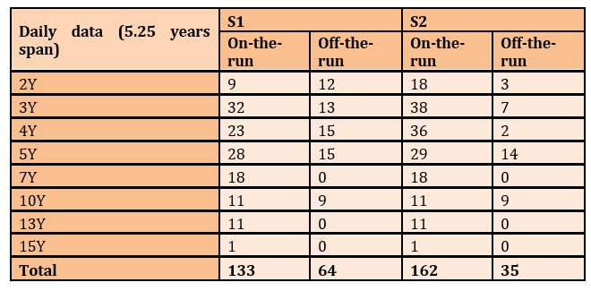
The second set of data includes auction results for ISIN reopenings[30] from the January 2015 – March 2019 period, for the same instruments aforementioned. We imported the aggregated results of primary market operations from the Refinitiv platform, but the MoPF also publishes them on their webpage, in the form of Official Results. During the selected period, the government issued debt at a wide range of maturities. In our paper, we included all those auctions held for ISINs with a residual maturity of 2, 3, 4, 5, 7, 10, 13 and 15 years respectively, so that we could cover all key maturities across the sovereign yield curve. Similarly to the method proposed by Cafiso, the Treasury bonds included in our study were further classified according to their “on-the-run”/”off-the-run” status. If not done properly, such classification can be a result of subjectivism, given there is no standard approach to determine the precise moment when a bond starts or ceases to become “on-the-run”. Moreover, such classification is aimed at providing information on how liquid an instrument is (as on-the-run bonds are associated with a high degree of liquidity, while off-the-run papers are generally illiquid, as they approach redemption). The standard approach is to consider a T-bond is “on-the-run” as soon as it is firstly issued. However, in countries where the same ISIN can be reopened several times –as it is the case of Romania- that specific instrument will not be liquid as soon as it is firstly issued, but after its outstanding amount is sufficiently high to enable dealers to trade it comfortably. Also, the standard approach pleads for considering a sovereign instrument to be “off-the-run” as soon as another instrument of the same initial maturity is issued. However, this behavior could lead to the exclusion from the “on-the-run” category of certain bonds that are still liquid. For example, if a government bond of initial maturity 7 years reaches residual maturity 6 years and a new 7-years T-bond is issued, it would be unrealistic to categorize the first as “off-the-run” (when actually it might still be highly liquid). In order to address the “on-the-run”/”off-the-run” categorization issue, we proposed 2 categorization methods, used them both and compared the results.
We named the first classification method (S1) as the Treasury Securities Fixing Component method and it implies that each new sovereign debt instrument newly issued which is component of the Treasury Securities (TS) Fixing[31] will be categorized as “on-the-run” until the next instrument of the same initial maturity is issued. As we have previously mentioned, one drawback implied by this method is that we might overlook some T-bonds that are still liquid. Regarding those debt instruments issued at maturities that are not TS Fixing maturities (1Y, 3Y, 5Y and 10Y), we will also consider them to be “on-the-run” until we have a new ISIN issued at that specific maturity or/and until its residual maturity equals the immediate lowest maturity which is part of the TS Fixing (e.g. T-bonds issued at 7 years will be considered “on-the-run” until their residual maturity equals 5- which is the immediate lowest TS Fixing maturity- or until a new 7-year T-bond is issued, only if the residual maturity of the first one has not went below the immediate lowest TS fixing maturity).
The second classification method (S2) –we named it the Treasury Securities Fixing Interval method- implies that a government bond will be categorized as “on-the-run” until its residual maturity equals the immediate lowest TS fixing maturity[32] (e.g. a T-bond with initial maturity 10 years will be considered “on-the-run” as long as its residual maturity is greater than 5 years, a T-bond with initial maturity 5 years will be classified as such until as long as its residual maturity is greater than 3 years etc.)
When comparing the 2 methods exposed above, with the Treasury Securities Fixing Interval method (S2) we have, indeed, 162 auctions of on-the-run securities as compared to only 133 auctions utilizing the other method, out of a total of 197 auctions considered. Further details on the comparison are exposed in below:
[1] Oprea, A., (2017), ‘The impact of MiFID II on the liquidity of fixed income instruments,’ Central Bank Journal of Law and Finance – National Bank of Romania. [Online], [Retrieved September 1, 2019], http://www.bnr.ro/Regular-publications-2504.aspx, 84
[2] Oprea, A., (2016), ‘An Analysis of Gold and Bond Market in the Context of Quantitative Easing Policy and Market Turmoil,’ Central Bank Journal of Law and Finance. [Online], [Retrieved September 1, 2019], http://www.bnr.ro/Regular-publications-2504.aspx, 118
[3] Gao, J., Jianjian, J. and Thompson, J. (2018), ‘The Impact of Government Debt Supply on Bond Market Liquidity: An Empirical Analysis of the Canadian Market,’ Bank of Canada – Staff Working Paper, 3, 19-22
[5] A reopening (or tap issue) of a bond allows the borrower to increase the amount in circulation of a previously issued bond, throughout a new auction
[7] Auctions of domestic bonds that are issued in foreign currency are typically announced in advance with a few working days
[8] The supplementary session for non-competitive offers (top-up session) is scheduled one working day after the reference auction
[9] On the Romanian government securities market, the standard maturities for T-bills are 6 or 12 months
[10] As per Regulation no. 7/2016 on the primary market of government securities on domestic market administrated by the National Bank of Romania (Romanian version only), Chapter III, Section 1, Article 16 and per Regulations on operations with government securities on domestic market approved through the order of the Ministry of Public Finances no. 2245/2016, Chapter III, Section 1, Article 15
[11] Not to be confounded with the non-competitive bids representing 15% of the same basis, which is the maximum amount that can be accepted at the supplementary session of non-competitive offers (SSON) that takes place the following working day
[12] As per Regulation no. 7/2016 on the primary market of government securities on domestic market administrated by the National Bank of Romania (Romanian version only), Chapter III, Section 1, Article 24, para. (1), para. (2) letter a)
[13] As per Regulation no. 7/2016 on the primary market of government securities on domestic market administrated by the National Bank of Romania (Romanian version only), Chapter III, Section 1, Article 21, para. (1), para. (2)
[14] The process of appointing a Primary Dealer is described in detail in Chapter II of Regulation no. 7/2016 on the primary market of government securities on domestic market administrated by the National Bank of Romania (Romanian version only)
[15] Arnone, M. and Iden, G. (2003), ‘Primary Dealers in Government Securities: Policy Issues and Selected Countries’ Experience,’ International Monetary Fund Working Paper28, 8-10.
[16] Fabozzi, F.J. (2007), Fixed Income Analysis Second edition (ed), John Wiley & Sons, Inc., Hoboken, New Jersey, 72.
[17] Fabozzi, F.J. and Mann, S.V. (2005), The Handbook of Fixed Income Securities Seventh edition (ed), The McGraw-Hill Companies, Inc., New York, 39-40.
[20] Cafiso, G. (2015) ‘Treasury auctions and secondary market dynamics. An analysis based on the MTS market for Italy.,’ University of Catania and CESifo Research Network, 14 (4), 4.
[22] This is the generally accepted formula for the BTC ratio, also used by the European Central Bank in the definition from their working paper (Beetsma, R., Giuliodori, M., Hanson, J. and Jong, de F. (2017), ‘Bid-to-cover and yield changes around public debt auctions in the euro area,’ ECB Working Paper No. 2056 / May 2017, 19).
However, in the case of Romania, the BTC formula is debatable, as the MoPF can choose to allocate an amount of government debt greater than the one announced in the issuance prospectus or make a partial allocation; so even though MoFP and news terminals such as Refinitiv calculate the BTC as a ratio between the amount offered and the amount allocated, there is a consensus among most Romanian dealers to calculate the BTC as a ratio between the amount offered and the amount announced by prospectus (which might differ from the allocated one). In this case, the ECB also advises to calculate the bid-to-cover ratio as the total amount bid over the target volume announced before the auction, because these can be taken as pre-determined in case of an analysis.
[23] Eisl, A., Ochs, C., Osadchiy, N., Subrahmanyam (2019), ‘The Linkage between Primary and Secondary Markets for Eurozone Sovereign Debt: Free Flow or Bottleneck?’ Vienna University of Economics and Business, Emory University and New York University. [Online], [Retrieved September 20, 2019], http://people.stern.nyu.edu/msubrahm/papers/Primary.pdf, 34.
[24] The procedure used by Cafiso (2015) is described in detail in his paper Treasury auctions and secondary market dynamics. An analysis based on the MTS market for Italy
[26] Meaning marginally higher than the secondary market bid yield, since a result lower than the ask level –even in the case of high BTC ratios- is a rare situation
[27] For ISIN ROGV3LGNPCW9, in the period between 18 September 2018 and 21 January 2019 we used bid yields as ask yields were not available to compute the mid quote
[28] Indicative market yields displayed on platforms such as Refinitiv or Bloomberg represent an accurate image of the approximate level of the firm prices at which transactions are executed. On the E-bond platform -which became the MoPF’s official market platform on the 1st of January 2017- the quotes displayed are firm. However, given the platform was launched after the start of the period considered in our paper, we have not used it as proxy for secondary market quotes. Also, although quotes on E-bond are firm, only primary dealers display them and perform trades at these yields, so we would ignore a significant number of players who might also be active within the government bond market. Therefore, we used indicative levels which we have considered to be more representative for the Treasury securities market as a whole.
[29] The hour limit for Delivery versus payment transactions is set at 16:45 as per SaFIR System Rules. SaFIR represents the financial instruments depository and settlement system operated by the National Bank of Romania.
[30] We excluded initial issuances and auctions of Treasury bills from our analysis, as for those government debt instruments there was no available data regarding market yields before the auction date, so insufficient to test a complete auction cycle
[31] Fixing Bid Rates and Fixing Offer Rates are established for Treasury bills issued at 6 months and 1 year, and benchmark Treasury bonds with initial maturities of 3, 5 and 10 years respectively, with the condition that they had been issued or reopened in the last 3 months prior to the calculation date of fixing rates, as per the Rules regarding the calculation of fixing rates issued by ACI Romania – The Association of Financial Markets
[32] To have a more precise image of both classification methods, the following scenarios are assumed: a 7-year T-bond is firstly issued, so it becomes on-the-run.
Scenario 1: A new 7-year T-bond is issued when the first T-bond still has a residual maturity above 5 years
With Method 1: the newly issued T-bond will be considered “on-the-run”, while the old one goes as “off-the-run”.
With Method 2: both debt instruments will be considered “on-the-run” until their residual maturity equals 5 years.
Scenario 2: A new 7-years T-bond is issued after the first T-bond residual maturity lowered below 5 years
With Method 1: the newly issued T-bond will be considered “on-the-run”, while the old one had already went “off-the-run” when its residual maturity lowered below 5 years.
With Method 2: the newly issued T-bond will be considered “on-the-run”, while the old one had already went “off-the-run” when its residual maturity lowered below 5 years.
Table 1: Auctions classification per status and maturity (daily frequency)
From our experience, in the case of the Romanian T-bond market, a potential V-inversed yield pattern around auction might be noticeable for a short period of time (+/- 1-2 days ante- and post-auction day). Thus, we will consider two sets of data:
daily market yields with an auction cycle comprising 5 days (yields in days t-2, t-1, t0, t1 and t2, where t0 accounts for the auction day)
intraday data with 30 minutes frequencies to observe how secondary market yields behave throughout the auction day
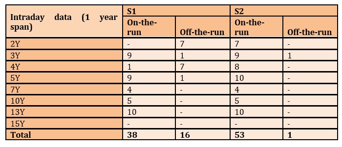
Table 2: Auctions classification per status and maturity (intraday frequency)
Empirical Results
Auction cycles and results from counting
As specified earlier in this paper, we considered a 5-day wide interval centered at the auction day to check for the auction cycle pattern and performed the analysis for both on-the-run and off-the-run Treasury securities, using both categorization methods explained earlier (S1 and S2). Similar to Cafiso (2015), the first stage of the analysis was performed by using variable , where represents the closing market mid yield from day t, t = {-2,-1, 0, 1, 2}, and t = 0 represents the auction day.
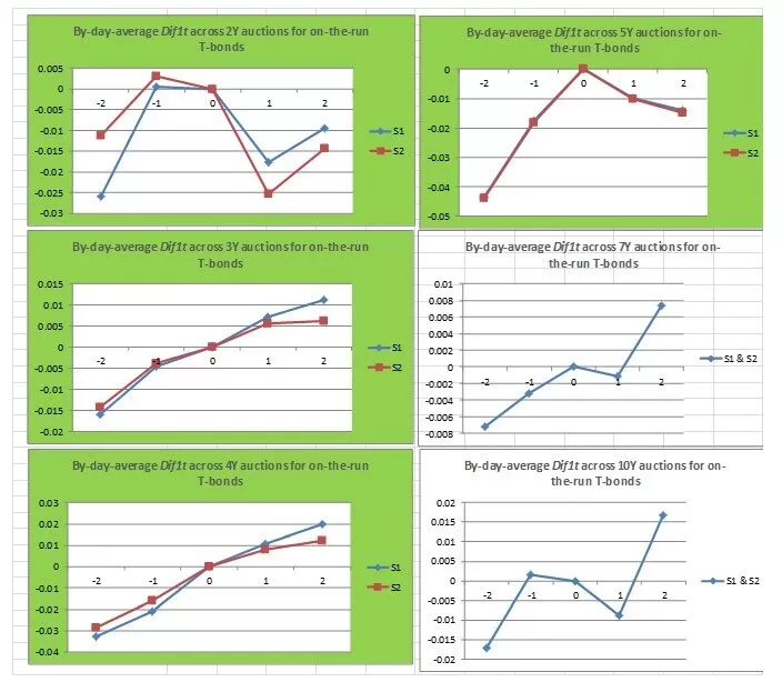
The values obtained are plotted in Figures 1 and 2 for each maturity[1] included in the study, and represent the by-day averages of across all the auctions.
[1] Our study includes data for all the ISINs auctioned in the period January 2015 – March 2019, with residual maturity of 2, 3, 4, 5, 7, 10, 13 and 15 years, thus covering all maturity segments across the sovereign yield curve
Fig 1. By-day-average for on-the-run T-bonds per auction cycle days (own computation from Refinitiv data)
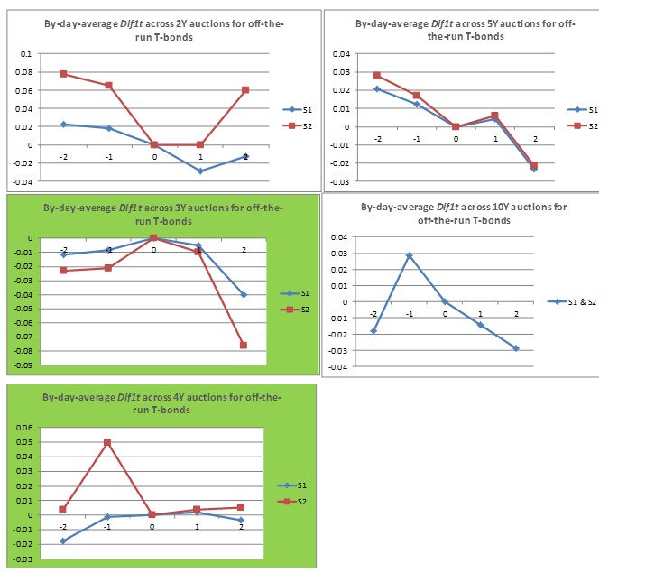
Fig 2. By-day-average for off-the-run T-bonds per auction cycle days (own computation from Refinitiv data)
With some exceptions, both on-the-run/off-the run categorization methods lead to similar results. However, for those categories for which we did not have a sufficient amount data, such as for off-the-run auctions categorized via the second method (S2), results might most probably have been compromised (e.g. over the period analyzed, there were only two auctions of 2-year off-the-run securities categorized as such by deploying the second method S2 versus 10 auctions resulted from method S1 and only one auction of 4-year off-the-run T-bonds versus 13 auctions in S1. There were no auctions of 7-, 13- and 15-year off-the-run Treasury securities, while in the case of 5-year debt instruments, both categorization methods described earlier lead to exactly the same results, meaning 11 auctions held for off-the-run T-bonds and 33 auctions conducted for on-the-run ones. In regards with the two categorization methods used, we conclude that besides the advantages that S2 brings by taking into account more liquid ISINs –and thus improving consistency among on-the-run estimations- it also carries the drawback of lowering the quality of the results obtained for the off-the-run government bonds. This is why we will not perform any further plot interpretations related to off-the-run bonds classified via the second categorization method.
Judging solely by the on-average plots, a perfectly inverted V-shaped auction cycle spreading throughout the 5-days window could only be observed for the on-the-run 5-year Treasury securities (with both categorization methods), and in the case of 3- and 4-year off-the-run papers. Most of the other maturities revealed what resembles more of a partial auction cycle pattern. For example, while the 3- and 4-years on-the-run instruments do display a yield increase of about 2-3 basis points from until the auction day, this movement is not followed by a yield reduction following the auction, but by a further increase at a slower pace-.
A deviation of the V-inversed yield pattern around auction days could also be noticed in the case of on-the-run 2-year T-bonds, as yields increased by about 2.5 basis points on average from to and decreased the day following the auction by approximately 2 basis points. However, in yields started to rise again. A similar behavior was observed for 7-year on-the-run government bonds but in that case the changes in the yield levels were insignificant (almost 1 basis point only).
As for those government securities that went off-the-run or for those of larger maturities –which are thus less liquid- plots also revealed only partial yield behaviors complying with an auction cycle pattern. For example, market yields for 13-year on-the-run securities displayed an increase of about 3 basis points at the auction day (compared to the day before), followed by a reduction of about 2.5 basis points in the day following the auction.
In terms of the amplitude of auction cycles, movements across all maturities included in the analysis varied between increases of about 3 basis points on average in the 1-2 days preceding the auction (including the auction day), followed by decreases of approximately the same size.
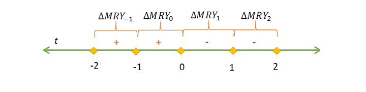
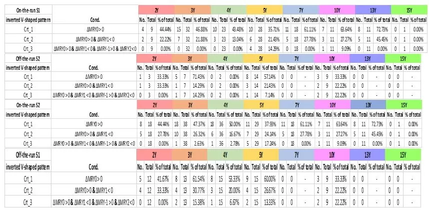
After observing yield patterns resulted from plots of by day average yield variations around primary market operations’ time, we proceeded with individual analysis and checked for those auctions where market yields behaved in a way described by the auction cycle, by actually counting those auctions using first differences , where t = 0 is the auction day. A V-inverted yield pattern implies positive changes in the MRY until the auction day inclusively, followed by a MRY decrease afterwards. Just as Cafiso (2015), we performed three stages of condition verifications, to split between those auctions where the inverted V-shaped pattern was more pronounced and prolonged and those which only accounted for partial auction cycle patterns.
In the first stage, we counted the auctions where > 0, meaning those for which an increase in yield was observed at the auction day. The second phase added another condition to the previous one, that 0, 0 and > 0. Results are summarized in Table 3 from the Appendix.
In 33% – 73% of the observations, securities across the sovereign yield curve exhibited an increase in the market yield at the auction day and only in 13% – 45% of the cases this increase was followed by a yield decrease in the day following the auction. Interestingly, when checking for the first differences, market yields corresponding to longer maturities displayed a more pronounced tendency to form an inverted V-shape pattern, at least for a 3-day wide window (from day to ): 13-year government securities revealed a positive yield variation at the auction day ( > 0) in 73% of the observations and a negative change afterwards ( < 0) in 46% of the times, while on-the-run 10-year papers displayed a yield increase at the auction day in 64% of the cases and a negative variation afterward in 27% of the times considered. By comparison, market yields corresponding to the 3-year segment and to the belly zone of the curve increased in only about 50%-60% of the cases at the auction day, but the width of the auction cycle was larger (on average 15% of the observations fulfilled all four conditions stated above jointly as opposed to 0% in the case of the 13-year T-bonds).
Results from regressions and intraday yield patterns during auction days
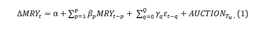
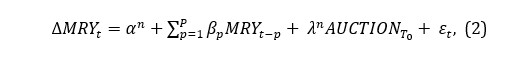
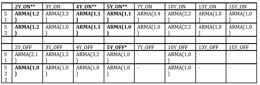
Although visual representations of by-day average yield variations across auctions were suggestive for an auction cycle pattern for at least some segments of maturities –especially the mid-term ones- an autoregressive model ARMA (p,q) was developed for each maturity and type of ISIN auctioned (on-the-run and off-the-run) –with results of ARMA estimations displayed in Table 4 from the Appendix. After the most suited model was found, we proceeded with the inclusion of dummy variables to check for the auction’s impact:
where dummies represent those days that form the auction cycle (T0 – the auction day, T1 – the day after the auction, T2 – 2 days after the auction, TM1 – the day before the auction and TM2 – 2 days before the auction). For each maturity included in the analysis -both on-the-run and off-the-run Treasury bonds- we performed 2 estimations to control for the auctions’ impact.
The first estimation (AUC_0) incorporates a dummy variable to account only for the auction day, so = 1 when t = 0 and = 0 in all the other days, when no government bond auction takes place for that specific maturity considered in the estimation. The second estimation (AUC_cycle) includes dummies for each day contained in the auction cycle: = 1 when t = -2 and 0 otherwise, = 1 when t = -1 and 0 otherwise, = 1 when t = 0 and 0 otherwise, = 1 when t = 1 and 0 otherwise and = 1 when t = 2 and 0 otherwise.
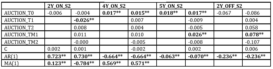
The estimation results exposed in Tables 5, 6 and 7 point towards confirmation of the inverted V-shape pattern in the case of on-the-run 2-year government securities and towards a partial auction cycle pattern for the 4- and 5-year on-the-run T-bonds.
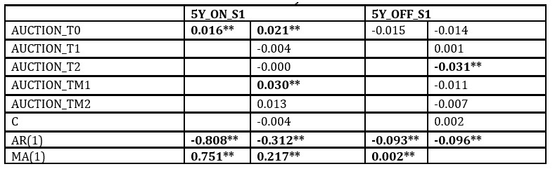
Table 5: Estimation results on the auction cycle for on- and off-the-run 5-year T-bonds (S1 method)
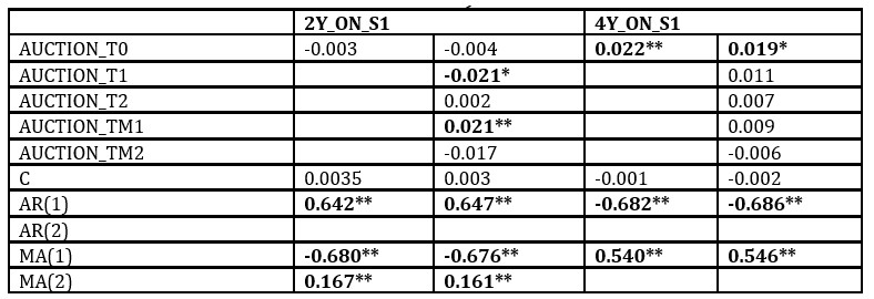
Table 6: Estimation results on the auction cycle for 2- and 4-year on-the-run T-bonds (S1 method)
Table 7: Estimation results on the auction cycle for on-the-run 2-, 4- and 5-year and off-the run 2-year T-bonds
More specifically, for those sovereign instruments maturing in 2 years’ time and which have been classified as “on-the-run” using the first categorization method (S1) explained earlier in this paper, the model revealed a 2.1 basis points increase in market yield in the day preceding the auction and a decrease of the same amplitude in the day following the primary market event, under a 10% (p-value = 0.07) and respectively 5% level of significance (p-value = 0.044). Under an even stronger significance level of 1%, on-the-run 5-year Treasury securities exhibited a 3 basis points yield increase in the day preceding the auction, followed by an additional 2 basis points increase at the auction day (both with p-value = 0.00); however, no subsequent decrease in yield could be observed under any level of statistical significance, so in this case we could only conclude for a partial auction cycle pattern. Also, in the case of on-the-run T-bonds with a residual maturity of 4 years, auction days were associated with increases of approximately 2 basis points in the market yield’s level (p-value = 0.014), but no variations could be attributed to the rest of days surrounding the auction. In terms of on-the-run/off-the-run categorization methods, both Treasury Securities Fixing Component method (S1) and Treasury Securities Interval method (S2) lead to similar results, excepting the off-the-run 2-year T-bonds category, which under S2 exhibited a statistically significant positive yield variation of nearly 8 basis points in the day preceding the auction. However, due to the reasons explained earlier in subchapter 5.1. we will not consider this result as relevant.
To assess the effect of Treasury auctions on the evolution of intraday market yields, we compared market quotes at different times during an auction day with those yields quoted at a considered “reference” hour. As stated previously, data consisted of intraday indicative quotes with 30 minutes frequency, from 9:00 a.m to 4:30 p.m, and the reference hour was fixed at 12 p.m[1]. Given the short period of time for which intraday data was available[2] and therefore the limited number of auctions held within one year –a statistic is provided in Table 2- the econometric analysis was performed on maturity segments corresponding to the short, medium and long-end of the sovereign yield curve and not for each residual maturity. Also, given the narrow range of off-the-run Treasury securities re-opened between April 2018 and March 2019, for the intraday assessment we only considered on-the-run T-bonds classified as such under the second categorization method exposed in chapter 4.
Similar to Fleming and Liu (2016)[3], we first calculated the average yield variation for each bond in the eight and a half-hour window considered for the intraday study, where the yield variation equals yield at t minutes away from auction minus the yield at auction time, where “t” takes values between -240 minutes (four hours before the auction) and 300 minutes (four and a half hour after the auction). 12:00 p.m. is considered to be the “auction time”, as it is a fixed and pre-determined point throughout an auction day, after which primary dealers are not allowed to submit or modify their auction offerings. Another approach would have been to consider the “auction time” as the time when auction results are published, given that information incorporated in the results often trigger additional movements on the yield curve. However, since the publication hour can vary significantly across auctions, this approach might have led to distorted results, especially because the sample of observations was not large enough to allow for the calibration of an optimal average publication hour.
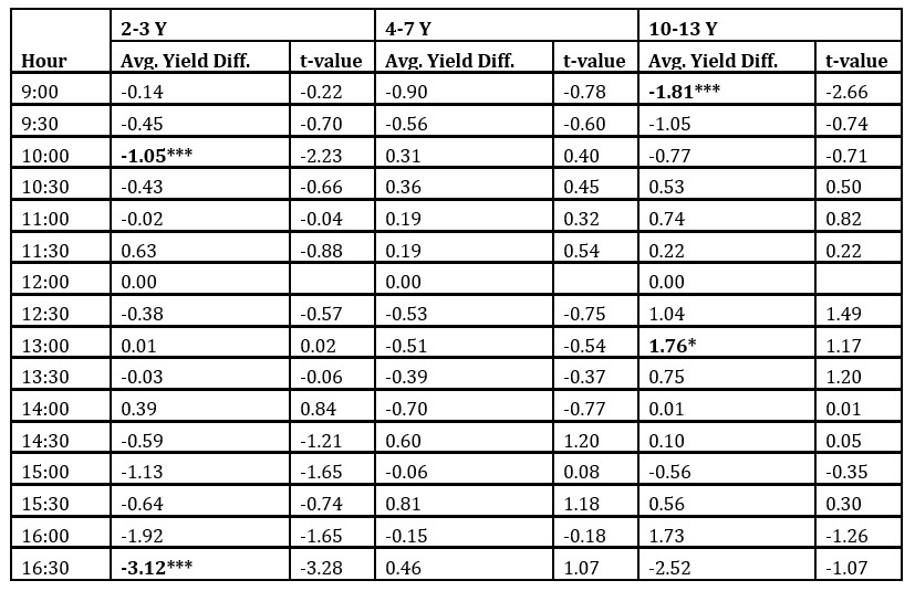
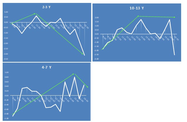
We first plotted the intraday average yield variations for each maturity and maturity segment (the 2-3-years segment accounted for the short end of the yield curve, the 4-7-years segment for the mid-zone and the 10-13-years group for the long-end). Afterward, we computed yield changes from t minutes away from auction to auction time and the corresponding standard errors, for each maturity segment (results are exposed in Table 8 from the Appendix).
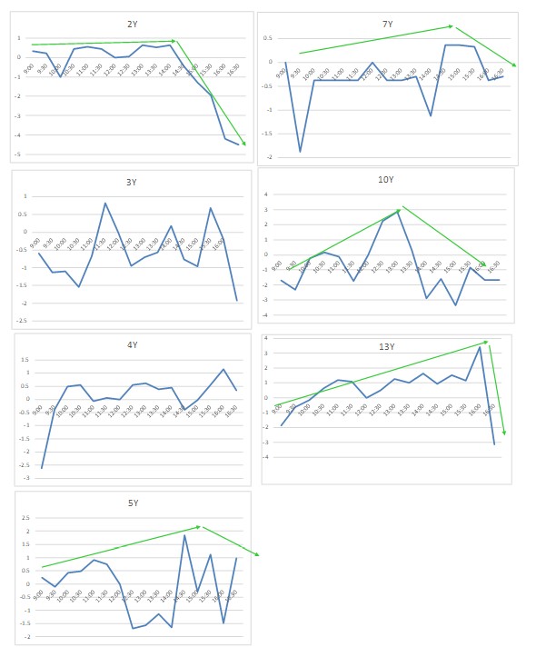
Judging by the plots displayed in Figures 3 and 4 from the Appendix, we observe that some V-inversed patterns do emerge in some cases. However, yield spikes are generally observed in the second half of the auction day, rather than near 12:00 p.m, sign that the “reference” hour requires further recalibration, as the inverted V-shape evolution of intraday yields –in case it emerges- is largely driven by auction results, and not by the time limit of primary dealers to submit bids. With the exception of on-the-run 10-year T-bonds, where corresponding market yields reveal a steep spike around 1 p.m., for the other maturities the spike in market quotes was observed between 2 and 4 p.m, which is precisely the time when auction results usually get published.
Interestingly, intraday 2-year yields exhibited low volatility in the first half of the auction day, followed by a sudden fall of about 4 basis points on average after 2 p.m. Going back to the 5-day wide window auction cycle, we remember that no statistically significant positive yield variation could be proved in day (no statistically significant increase in yield at the auction day compared to the day before). However, when looking at the entire 5-day cycle for this particular maturity, we do observe an increase in yield (which also proved to be significant under a 10% level of significance with p-value = 0.07) in the day preceding the auction compared to the day before and a decrease of approximately the same amplitude in day (the day following the auction). This hints us to consider that even though auction days might be characterized by low levels of volatility, the indicative market quotes might have already started their upward positioning 1-2 days before the primary market event.
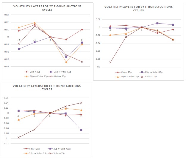
Auction cycle in respect to different volatility regimes
In times of market turmoil and increased volatility, investors might demand additional risk premia to hold specific instruments. In the case of sovereign bonds, if the theory regarding the limited risk-bearing capacity of dealers holds, then they would have to sell more bonds before the auction, to cover for the additional risk associated with buying new ones from the primary market. Eventually, this would translate into a more pronounced effect of auctions on market yields and thus into a higher amplitude of the auction cycle. Beetsma et al. (2014), Cafiso (2015) and Eisl and Ochs (2019) all have documented the connection between volatility and bond auctions. The first study delivers some results that are suggestive for the aforementioned connection, respectively that in times of increased yields volatility and widening of CDS spreads, the auction cycle is deeper. Such pattern is in line with the inventory-adjustments that dealers -due to their limited risk-bearing capacity- make in their portfolios prior to the auction. Eisl and Ochs (2019) go further with the study of this interdependence and find that the extent to which primary dealers adjust their positions is also related to the degree of riskiness and liquidity of the bond being auctioned. More specifically, the issuance of a more risky bond requires dealers to sell-off more of their risky inventory (which, in turn, increases the magnitude of the auction cycle[4]), while a more liquid auctioned Treasury security allows them to adjust portfolios more smoothly.
Again, in order to assess the interdependence between volatility and auction effects on secondary market yields, we followed the path of Cafiso (2015) and started by defining four layers of volatility and assigning each auction to a specific volatility layer. Only those ISINs with residual maturity of 2, 4 and 5 years (so only for those maturities that displayed a V-inversed yield pattern or at least a partial pattern throughout the 5-day wide window auction cycle) were included in this analysis. At first, the standard deviation of market yields over the 3 days preceding the auction (including the auction day) was computed as a proxy for the historical volatility, and a specific volatility value was attributed to each auction. Subsequently, four layers of volatility were defined: 1) below the 25th percentile, 2) between the 25th and the 50th percentile, 3) between the 50th and the 75th percentile and 4) above the 75th percentile and each auction was assigned to a volatility layer, according to its volatility value[5]. After that, variable already defined in subchapter 5.1 as the difference between and was calculated for each t within the auction cycle window, and its values were averaged across auctions belonging to the same volatility layer. By-day average values of per volatility layers are plotted in Figure 5.
[1] It represents the time limit for Primary Dealers to submit their bids at a reference auction
[2] In Bloomberg and Refinitiv, intraday quotes for government yields are only available for 1 year behind the interrogation date
The inverted V-shaped evolution of yields for 2-year T-bonds emerged under the 2nd and 4th layer, so in times of low-to-moderate volatility and also in times of increased variations of market yields. A partial auction cycle marked by yield decreases in T+1 was observed under all four volatility regimes. However, yield declines registered in times of moderate and high volatility were more pronounced than those marked in a low volatility environment.
For Treasury securities of 4- and 5-years residual maturity, we observe and interesting behavior of yields, consistent with the limited risk-bearing capacity of dealers. As we have mentioned earlier in this paper, the 4- and 5-year T-bonds exhibited an increase in yield of about 4 basis points on average from day to , where represents the auction day. However, when analyzing the volatility plots, we observe that these increases were registered only under 2 regimes: the moderate and the high volatility one. Also, the movements were of larger amplitude in times of high volatility (about 8 basis points average increase in the yield level from to ) compared to approximately 2 basis points increases in times of moderate market variations. No specific differences in the yield pattern could be observed between the four volatility layers for the days following the auction.
After observing yield patterns from plotting by-day average yield variations across different layers of volatility, we performed an additional analysis which included all the ISINs auctioned between January 2015 and March 2019 with residual maturities of 2-, 4- and 5-years throughout Markov-switching estimations as in Hamilton (2008). This time only two volatility regimes were considered (n=2), corresponding to a low and a high volatility environment, respectively. Thus, the equation for the Markov-switching estimations is similar to equation 1:
where MA terms are not included and the AR terms deployed are the same found in our first estimations of ARMA (p,q) models. is the coefficient of interest of these estimations, as it quantifies the effect of auctions on the level of market yield, when those auctions are assigned to two different volatility regimes (n = 1, 2). One thing to note here is that only observations at the auction day were considered in this analysis, so dummy variable = .
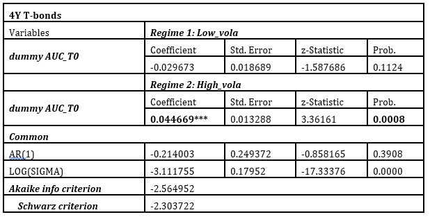
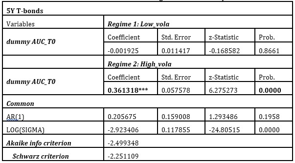
From the Markov-switching estimations, the higher impact of T-bond auctions over market yields in times of increased volatility proved statistically significant only for the 4- and 5-year government securities. This finding –which is also consistent with the observation of Eisl and Ochs (2019)[1]– is relevant given the higher liquidity at the belly of the yield curve, and thus the particularity of these T-bonds to get sold-off first by primary dealers, in order to minimize the effect that bond auctions determine on their portfolios. Such effect of auctions was more pronounced in the case of 5-year T-bonds (coefficient λ = 0.36 under the high volatility regime with p-value = 0.0000 compared to λ = 0.044 in the high volatility environment with p-value = 0.0008 for the 4-year sovereign debt instruments).
Most probably, the aforementioned deeper impact was caused by the higher differences between the low and high volatility regimes of the two maturities: while the 4-year Treasury securities exhibited daily yield variations of at last +/- 13-15 basis points at the auction day, the maximum yield change in the case of 5-year T-bonds was of up to 35 basis points[2].
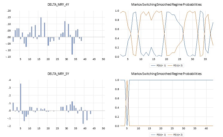
The estimation output for the two residual maturities mentioned above is available in Tables 9 and 10, along with the plots representing the corresponding smoothed regime probabilities and the daily yield variations in Figure 6 from the Appendix.
On the whole -in terms of statistically significant results- in times of increased volatility on the sovereign bond market, the impact of auctions over market quotes proved stronger for those T-bonds corresponding to the belly zone of the yield curve.
Conclusions
The aim of this study was to check for the existence of a specific pattern in the level of market yields of Romanian government bonds around auction days. So far, the auction cycle has representedone of the most widely accepted hypotheses under which certain yield movements might get an explanation when primary market operations take place. Mainly due to the limited risk-bearing capacity of primary dealers, they tend to make portfolio adjustments before submitting their bids at an auction, so they sell part of their holdings in order to allow for a potential intake of risk, from the new T-bonds they might acquire throughout the primary market event. Such adjustments should then lead to an inverted V-shape pattern of market yields, with the maximum yield registered at the auction day.
Unlike other papers from the literature, for the Romanian sovereign bond market we integrated both intraday and lower frequency data analysis and checked for the formation of the auction cycle across the two. Last, given the higher degree of risk associated with acquiring bonds in times of increased market volatility, we check for the amplitude of the auction cycle under different layers of volatility.
To our awareness, this is the first documented paper assessing the interdependence between primary market operations and market yields for the Romanian Treasury securities market.
Based on the specificities of the local bond market, a 5-day wide window centered at the auction day was considered for the daily frequency analysis, including on-the-run and off-the-run T-bonds auctioned between January 2015 and March 2019. Both by-day-average plots of yield variations within the auction window and the econometric estimations where dummy variables were included to account for the auction day and for the +/- 2 days around the auction day confirmed the formation of a V-inversed shape of market yields in the case of on-the-run 2-year government securities and of a partial auction cycle pattern for the 4- and 5-year on-the-run T-bonds. More specifically, for those sovereign instruments with a residual maturity of 2 years, the model revealed a statistically significant yield increase of about 2 basis points in the day preceding the auction (with a flat evolution at the auction day) and a decrease of the same amplitude in the day following the primary market event. On-the-run 5-year Treasury securities exhibited a 3 basis points yield increase in the day preceding the auction, followed by an additional 2 basis points increase at the auction day, thus a total increase of about 5 basis points throughout the 2 days preceding the auction; however, no subsequent decrease in yield could be observed under any level of statistical significance, so in this case we could only conclude for a partial auction cycle pattern. Also, in the case of on-the-run T-bonds with a residual maturity of 4 years, auction days were associated with increases of approximately 2 basis points in the level of the market yield, but no variations could be attributed to the rest of the days surrounding the auction.
To assess the impact of Treasury auctions on the evolution of intraday market yields, we compared indicative market quotes at different times during an auction day with those quoted at a “reference” hour, which we considered as the “auction time”. For homogeneity purposes, this was established at 12:00 p.m, as it is a fixed, pre-determined point throughout an auction day, after which primary dealers are not allowed to modify their already submitted offerings or send new ones. Here, although the inverted V-shape pattern did emerge in some cases, yield spikes were generally observed in the second half of the auction day, rather than near 12:00 p.m, signaling that the “reference” hour requires further recalibration, as the V-inversed evolution of intraday yields –in case it emerges- is largely driven by auction results, and not by the time limit of primary dealers to submit bids.
Interestingly, intraday 2-year yields exhibited low volatility in the first half of the auction day, followed by a sudden fall of about 4 basis points on average after 2 p.m. Looking back at the 5-day wide window auction cycle, we remember that even though no statistically significant positive daily yield variation could be proved at the auction day for this particular maturity, an increase in yield was still confirmed in the day preceding the auction and also a decrease of approximately the same amplitude in the day after the auction. Such finding made by integrating intraday observations with lower frequency data, hinted us to consider that even though at first glance auction days appear characterized by low levels of volatility, market yields might have already started their upward positioning 1-2 days before the primary market event, and thus an inversion has the potential to be triggered.
Eventually, we checked for the amplitude of the auction cycle under different volatility environments. We averaged the daily yield variations within the auction cycle and plotted them per layers of volatility. At first, we considered -such as in Cafiso (2015)- four volatility layers, grouped from low to high volatility, based on the quartiles of the distribution of auctions’ volatility values, calculated as the standard deviation of the market yield in the last 3 days (including the auction day). In the second stage, we performed Markov-switching estimations under 2 volatility regimes (low and high, respectively).
The amplitude of the auction cycle proved to be more pronounced in times of increased market volatility for those government securities with a residual maturity of 4- and 5-years. The results is relevant given the higher liquidity at the belly of the yield curve, and thus the particularity of these debt instruments to get sold-off first by primary dealers, in order to minimize the effect that bond auctions determine on their portfolios. Our interpretation is also consistent with the research of Eisl and Ochs (2019), who demonstrate that the extent to which primary dealers adjust their positions is related –among other things- to the degree of riskiness and liquidity of the bond being auctioned.
Acknowledgment
The opinions expressed in this research paper are those of the author and do not necessarily reflect the views of the institutions mentioned in the paper, nor do they engage them in any way.
References
Arnone, M. and Iden, G. (2003), ‘Primary Dealers in Government Securities: Policy Issues and Selected Countries’ Experience,’ International Monetary Fund Working Paper28, 8-10.
Beetsma, R., Giuliodori, M., Hanson, J. and Jong, de F. (2017), ‘Bid-to-cover and yield changes around public debt auctions in the euro area,’ ECB Working Paper No. 2056 / May 2017, 19.
Cafiso, G. (2015) ‘Treasury auctions and secondary market dynamics. An analysis based on the MTS market for Italy.,’ University of Catania and CESifo Research Network, 4-18.
Eisl, A., Ochs, C., Osadchiy, N., Subrahmanyam (2019), ‘The Linkage between Primary and Secondary Markets for Eurozone Sovereign Debt: Free Flow or Bottleneck?’ Vienna University of Economics and Business, Emory University and New York University. [Online], [Retrieved September 20, 2019], http://people.stern.nyu.edu/msubrahm/papers/Primary.pdf, 34.
Fabozzi, F.J. (2007), Fixed Income Analysis Second edition (ed), John Wiley & Sons, Inc., Hoboken, New Jersey, 72.
Fabozzi, F.J. and Mann, S.V. (2005), The Handbook of Fixed Income Securities Seventh edition (ed), The McGraw-Hill Companies, Inc., New York, 39-40.
Gao, J., Jianjian, J. and Thompson, J. (2018), ‘The Impact of Government Debt Supply on Bond Market Liquidity: An Empirical Analysis of the Canadian Market,’ Bank of Canada – Staff Working Paper, 3, 19-22
Oprea, A., (2017), ‘The impact of MiFID II on the liquidity of fixed income instruments,’ Central Bank Journal of Law and Finance – National Bank of Romania. [Online], [Retrieved September 1, 2019], http://www.bnr.ro/Regular-publications-2504.aspx, 84
Oprea, A., (2016), ‘An Analysis of Gold and Bond Market in the Context of Quantitative Easing Policy and Market Turmoil,’ Central Bank Journal of Law and Finance. [Online], [Retrieved September 1, 2019], http://www.bnr.ro/Regular-publications-2504.aspx, 118
Regulation no. 7/2016 on the primary market of government securities on domestic market administrated by the National Bank of Romania (Romanian version only), Chapter III, Section 1, Article 16, Article 21, para. (1), para. (2)
Regulations on operations with government securities on domestic market approved through the order of the Ministry of Public Finances no. 2245/2016, Chapter III, Section 1, Article 15
[2] That market movement corresponded to a period of increased volatility in the first week of October 2018, when the borrowing costs on the bond market were experimenting an upward pressure that lead to a surge in yields of about 30-40 basis points across the sovereign yield curve in a couple of days. Via Markov-switching estimations, auctions held in that period were assigned the high volatility regime.
Appendix
Table 3: Results from counting per auction cycle criteria
Table 4: ARMA specifications for
Table 8: Yield changes around auction time per maturity segment
Note: The table shows average (mid) yield changes from t minutes from auction to time of auction
on the secondary market per maturity segment corresponding to the short, medium and long-end of the sovereign yield curve between April 1, 2018 and March 31, 2019. *, **, and *** denote significance at the 10, 5, and 1% levels using a t-test of zero means.
Fig 3. Yield differences t away from the reference hour around Treasury auction
Fig 4. Yield differences t away from the reference hour around Treasury auctions per maturity segments
Table 9: Results from Markov-switching estimations for 4-year T-bonds
Table 10: Results from Markov-switching estimations for 5-year T-bonds
Fig 4. Day-on-day yield differences and corresponding Markov-Switching Smoothed Regime Probabilities for 4- and 5- T-bonds around Treasury auctions (where P(S(t)=1 represents the probability associated with the low volatility regime, and P(S(t)=2 represents the probability associated with the high volatility regime)