The Bucharest University of Economic Studies Bucharest, Romania
Volume 2025,
Article ID 853501,
Journal of Financial Studies and Research,
21 pages,
DOI: https://doi.org/10.5171/2025.853501
Received date: 30 September 2025; Accepted date: 31 December 2025; Published date: 17 February 2025
Cite this Article as:
Cristina – Elena BEJENARU (2025)," Examining Behavioral Deviations in Economic Forecasts: A Study of the Eurozone and CEEC", Journal of Financial Studies & Research, Vol. 2025 (2025), Article ID 853501, https://doi.org/10.5171/2025.853501
Drawing on behavioral insights and heuristics, this study demonstrates the ways in which more realistic decision-making diverges from the classic homo economicus model. Employing the New-Keynesian behavioral model proposed by De Grauwe (2012, 2019) and parameters from Jang and Sacht (2016), the analysis reveals a superior fit for observed fluctuations in output and inflation across the Eurozone and Central and Eastern European economies compared to models assuming strictly rational expectations. The findings also indicate non-normal distributions in the output gap and notable serial correlation in both inflation and output, underscoring the pivotal influence of market sentiment – captured by an animal spirit index – on macroeconomic volatility.
Recent research in economics, combined with insights from psychology, has revealed significant deviations in human behavior from the traditional economic hypothesis of homo economicus. Matthew Rabin (2002) and Stefano DellaVigna (2009) distinguish three principal categories of deviations from the standard neoclassical model: non-standard preferences (such as social preferences and time preferences), non-standard beliefs (such as overconfidence), and non-standard decision-making processes (such as heuristics and framing).
Traditional economics assumes that individuals act solely to maximize their self-interest. However, as early as 1759, Adam Smith highlighted the altruistic dimension of human nature in his work, The Theory of Moral Sentiments. An example of non-standard preferences is the concept of social preferences, where individuals act not only in their own self-interest but also in the interest of others, demonstrating behaviors such as cooperation and reciprocity. Numerous experimental studies have shown that individual utility can, in fact, derive from the act of giving, indicating that satisfaction is not solely driven by self-interest.
Intertemporal choice is critical to decisions related to saving, work effort, education, nutrition, and healthcare. This concept refers to how individuals make choices that affect both the present and the future, with current decisions influencing future opportunities. Traditional economic models typically analyze intertemporal choice using the discounted utility framework, which assumes individuals evaluate pleasure and pain consistently over time, typically using an exponential discount function. However, empirical studies have demonstrated that individuals often prefer smaller immediate rewards over larger delayed ones when the payoff is near-term, while showing greater patience for larger rewards when the payoff is in the distant future. To address these inconsistencies, Loewenstein and Prelec (1992) and Frederick, Loewenstein, and O’Donoghue (2002) proposed replacing the exponential discount factor with a hyperbolic function, which better captures these behavioral tendencies. Similarly, Thaler (1981) concluded that the preference for immediate gratification, at the expense of long-term consumption and savings, can be attributed to a lack of self-control.
One of the most prominent theories integrating psychological aspects of human behavior is Prospect Theory, proposed by Daniel Kahneman and Amos Tversky (1979) as an alternative to Expected Utility Theory. Prospect Theory describes decision-making under conditions of uncertainty and risk through two functions: the value function and the decision-weighting function. Losses are felt more intensely than gains (loss aversion), and are evaluated with a convex function, while gains are evaluated with a concave function. The decision-weighting function highlights individuals’ tendencies to underestimate small probabilities and overestimate larger ones.
These insights demonstrate that economic agents operate with bounded rationality. First introduced by Herbert Simon (1959), the concept of bounded rationality was further explored by Kahneman and Tversky. They argued that individuals rely on heuristics and are subject to biases that affect decision-making under uncertainty. Heuristics are mental shortcuts, derived from experience, that simplify complex problems and allow individuals to make quick decisions. In Thinking, Fast and Slow (2011), Kahneman differentiates between two modes of thinking: one that is fast, intuitive, and based on heuristics, and another that is slow, analytical, and deliberate.
In recent years, researchers have incorporated behavioral economics hypotheses into macroeconomic models to better capture the complexity of economic phenomena. Many have relaxed the assumptions underlying Neo-Keynesian Dynamic Stochastic General Equilibrium (DSGE) models or introduced new hypotheses altogether.
A critical assumption in macroeconomic models is how individuals form expectations, which guide their decision-making. DSGE models typically operate under the rational expectations hypothesis (Muth, 1961). However, by relaxing this assumption, Paul De Grauwe (2012) developed a Neo-Keynesian behavioral model in which agents form expectations about future inflation and output using two simple rules (heuristics): the fundamentalist rule and the extrapolation rule. Agents engage in adaptive learning, choosing the rule that has performed best in the past. A key feature of De Grauwe’s model is that agents exhibit optimism during economic booms and pessimism during recessions (animal spirits). Unlike the classical Neo-Keynesian model, where economic fluctuations are largely driven by exogenous shocks, De Grauwe’s model suggests that business cycle fluctuations can result from oscillations in animal spirits.
In this paper, we compare the key characteristics of variables generated by the Neo-Keynesian behavioral model, as proposed by Paul De Grauwe (2019) and calibrated using parameters estimated by Tae-Seok Jang and Stephen Sacht (2016), with empirically observed variables such as the output gap and inflation in the Eurozone and four Central and Eastern European countries (Romania, Hungary, Poland, and Czechia). Our findings demonstrate that the behavioral model better replicates the observed empirical dynamics compared to the Neo-Keynesian model with rational expectations.
Methodology
The Neo-Keynesian behavioral model
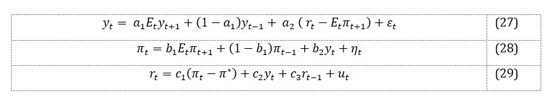
The Neo-Keynesian (NK) behavioral model (BH), proposed by Paul De Grauwe[1], is based on three fundamental equations: the aggregate demand equation, the aggregate supply equation, and a Taylor-type rule that describes the behavior of the central bank.
Aggregate demand equation:
where represents the output gap, , is the nominal interest rate și is the inflation rate. describes the expectations the operator formed in the context of bounded rationality.
Aggregate supply equation:
Taylor-type rule:
where represents the inflation target; , , , , , și re the constant coefficients associated with the variables, and and are the error terms, describing potential shocks that impact the economy, which follow a normal distribution with zero mean and constant variance.
Agents’ Expectations
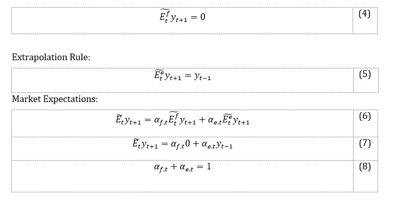
Economic agents use two simple rules for forecasting the output gap and inflation rate, based on a trial-and-error learning strategy. Through this approach, they periodically evaluate the forecasting rules and choose the one that performs best. Additionally, the presence of these two rules introduces heterogeneity into the model, as agents interact and influence each other. The two rules are the fundamentalist rule and the extrapolation rule. In the first case, agents know the equilibrium value of the output gap, and their expectations align with it. In the second case, expectations are formed based on the previous value of the variable.
The mechanism for selecting the output gap forecasting rule
Fundamentalist Rule:
where and represent the probabilities that agents will use the fundamentalist rule and the extrapolation rule, respectively.
The selection of the forecasting rule is based on a trial-and-error learning strategy, where agents continuously evaluate the performance of the forecasting rule they are using.
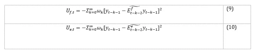
We define the utility (performance) resulting from the use of the forecasting rules as:
where and are the utilities of each selected rule, and represents the geometrically decreasing weight, indicating the tendency of individuals to forget: smaller weights are allocated to deviations from more distant periods compared to those from the recent period.
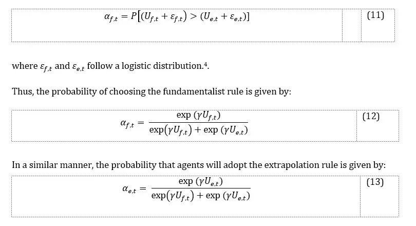
To evaluate the performance of the forecasting rules, discrete choice theory is applied[2]. According to specialized studies[3], individual decisions may be influenced by various factors, such as the present mood or state of mind, which can be reflected by incorporating a random component. Thus, the probability of choosing the fundamentalist rule becomes:
Equation (12) indicates that, as the relative performance of the fundamentalist rule improves, the probability of agents using this rule to forecast the output gap increases.
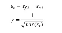
The parameter γ represents the intensity of choice and is dependent on the variance of the random components.
We define
When tends toward infinity, γ approaches zero; in this case, = 0,5, meaning the choice is purely stochastic. Conversely, when γ tends toward infinity, the variance of the random component approaches zero (utility becomes purely deterministic), and will be either 1 or 0. The parameter γ can be interpreted as the agents’ willingness to learn by evaluating the past performance of the rules through a trial-and-error process. This helps them avoid systematic mistakes and adapt their behavior by switching the rule they use.
The Mechanism for Selecting the Inflation Forecasting Rule
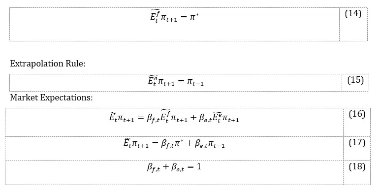
Fundamentalist Rule:
The probability that agents will use the fundamentalist/extrapolation rule is given by:
The rules that describe how agents form expectations regarding the output gap and inflation rate are independent, with no predisposition for agents to select one rule more frequently than the other.
Animal Spirit
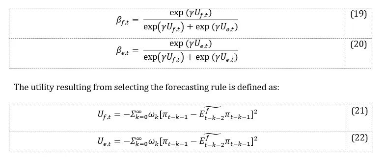
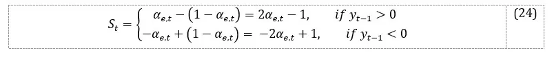
We define a market sentiment index, referred to as the animal spirit, which reflects the degree of optimism/pessimism among agents:
where is the animal spirit index, which can take values between ±1, as follows:
When , agents using the extrapolation rule anticipate a positive output gap.[5];
Since the fundamentalists’ forecast tends toward zero (the equilibrium level of the output gap), they will be considered pessimists. When the proportion of optimists exceeds that of pessimists[6], becomes positive, and there is a possibility that, through a contagion effect, all agents become optimistic, leading to . If the proportions of agents using each rule are equal (), the animal spirit is neutral, and .
When , those using the extrapolation rule anticipate a negative output gap. When the proportion of pessimists exceeds that of optimists, becomes negative, and there is a possibility that all agents become pessimistic, leading to .
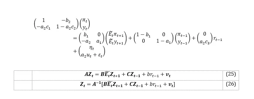
We rewrite the equations as follows:
Solving the Model
We obtain the solution to the model by substituting equation (3) into equation (1):
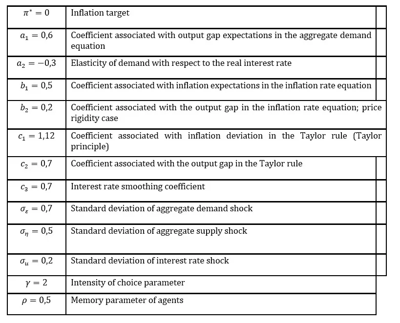
Parameters of the model
The parameters used for simulating the model are derived from the simulated method of moments estimated by Jang and Sacht (2016), who empirically evaluated De Grauwe’s model using Euro Area data from 1975Q1 to 2009Q4 while comparing its performance to the standard model with rational expectations. Their findings reveal that the model-generated auto- and cross-covariances of the output, inflation, and nominal interest rate gaps effectively approximate the empirical second moments.
Table 1: Parameters
Source: Parameter values are taken from “Animal Spirits and the Business Cycle: Empirical Evidence from Moment Matching” by Tae-Seok Jang and Stephen Sacht, with the main difference being that the values for the agents’ memory and intensity of choice parameters are retained as in De Grauwe and Ji (2019).
The system has a solution if the determinant of matrix is non-zero: . The solution for e is obtained by substituting the values of given by system (26) into equation (3). Due to the nonlinear nature of the system, numerical methods are employed to analyze its dynamics. We calibrate the model by selecting numerical values for its parameters (Table 1).
Neo-Keynesian Model with Rational Expectations
In this section, we introduce the Neo-Keynesian model with rational expectations and subsequently compare the key results obtained from the estimations of the behavioral model and the rational expectations model.
The RE model comprises three equations: the aggregate demand equation, the aggregate supply equation, and a Taylor-type rule:
The variable notations are as previously described, except for expectations () which in this case are formed exclusively rationally, as described by the fundamentalist rule. The parameter values are sourced from Tae-Seok Jang and Stephen Sacht (2016) for the hybrid RE case, which incorporates structured inertia into the model[7]. The models are simulated over 10.000 periods using Matlab[8]. The model is calibrated on a quarterly time scale. The error terms of the three main equations follow a normal distribution and are independently and identically distributed. The endogenous variables – the output gap, inflation rate, and nominal interest rate – are expressed as deviations from their equilibrium values, with initial values set to zero.
Results
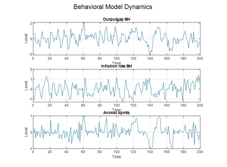
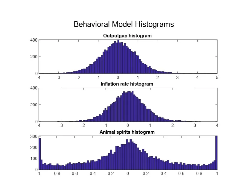
This section presents the key results obtained from the behavioral model and compares them with those derived from the rational expectations model. To illustrate the dynamics of the variables of interest (Figure 1), a representative sample of 200 observations (quarters) was selected. The histograms displayed correspond to variables with 10.000 observations.
Figure 1: NK BH Model: dynamics of the output gap, animal spirit, and inflation rate
Figure 2: NK BH Model: histograms of the output gap, animal spirit, and inflation rate
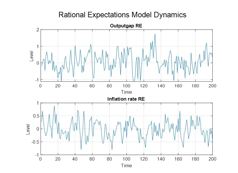
Figure 3: NK RE Model: dynamics of the output gap, animal spirit, and inflation rate
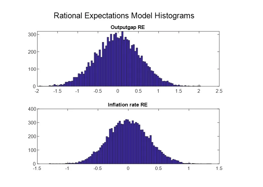
Figure 4: NK RE Model: histograms of the output gap, animal spirit, and inflation rate
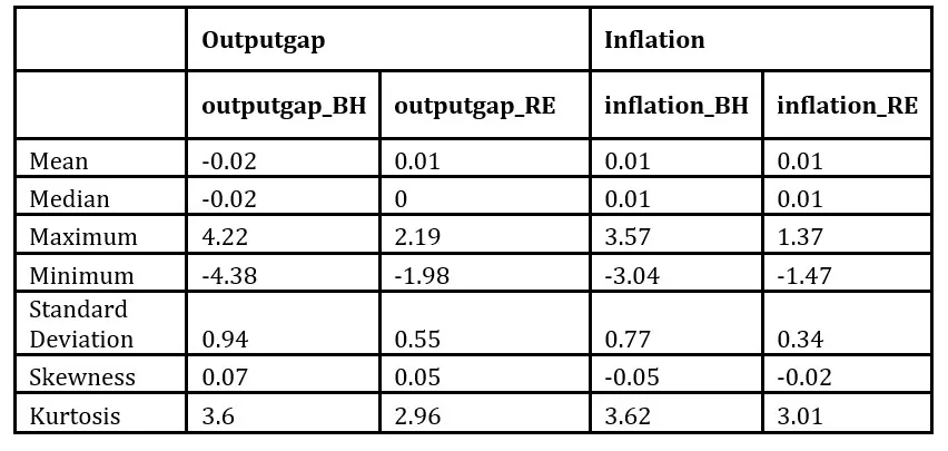
Table 2: Statistical Characteristics for output gap and inflation in BH and RE models
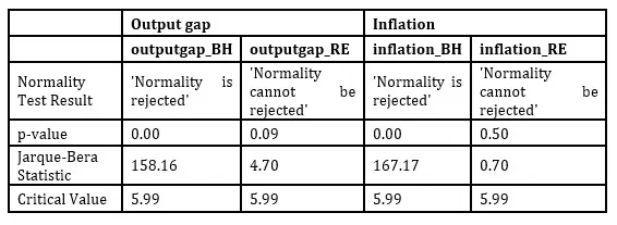
Table 3: Jarque-Bera Test Results for output gap and inflation in BH and RE models
From Figure 1, we can observe that the model endogenously generates fluctuations of optimism and pessimism in the market, which amplify due to the self-fulfilling nature of agents’ expectations, leading to situations of widespread optimism () or pessimism (). Furthermore, a high correlation between the output gap and animal spirits is evident, reaching a coefficient of 0.83. This correlation is explained by the self-fulfilling nature of expectations: a higher proportion of optimistic agents leads, according to equation (1), to an increase in aggregate demand, which in turn generates a rise in the proportion of optimistic agents.
Additionally, Figure 2 presents histograms of the main variables analyzed, revealing that the output gap does not follow a normal distribution but rather a leptokurtic one with a kurtosis index of 3.6 (Table 2). This characteristic arises from the distribution of the animal spirit variable, whose histogram shows a concentration of values around zero, suggesting that most of the time the situation is normal, without extreme events. Simultaneously, there is a concentration of values at the tails of the animal spirit distribution, which accounts for the heavy tails observed in the output gap distribution. In contrast to the classical NK model (Table 3), this non-normality of the output gap distribution is generated by the behavioral model because of fluctuations in economic agents’ sentiment, rather than by introducing exogenous shocks with a pre-specified abnormal distribution. The obtained results, which will be discussed further, are consistent with the observed characteristics of the output gap and inflation in several countries.
To compare the characteristics of the variables obtained from the simulated models with those empirically observed, we analyze the dynamics, histograms, and perform the Jarque-Bera test for the output gap series of the Euro Area, the Czech Republic, Hungary, Poland, and Romania over the period from Q1 1995 to Q2 2024 (obtained using a Hodrick-Prescott filter with lambda 1600) and for the annual inflation rate series from Q1 1997 to Q2 2024 (based HICP index). The source of all data was Eurostat database. For verification purposes, we excluded the pandemic crisis period, as it could distort the main characteristics. However, the results obtained both with and without that period are similar.
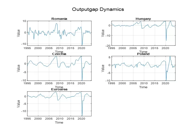
Figure 5: Output gap dynamics
Figure 6: Output gap histograms
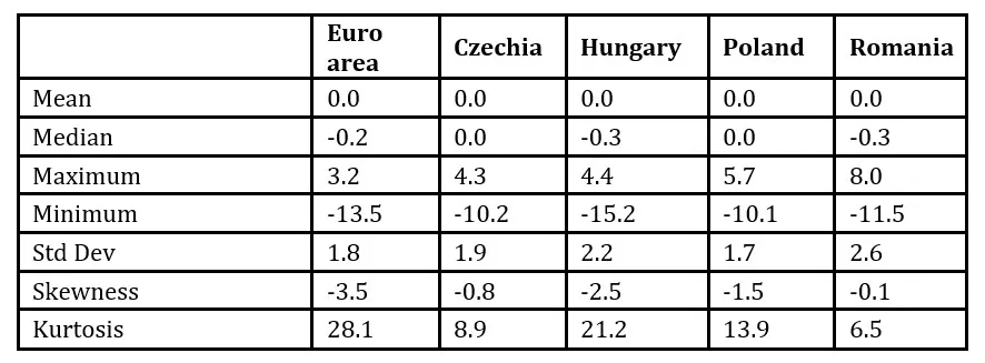
Table 4: Statistical Characteristics for output gap
Table 5: Jarque-Bera Test Results for output gap
Figures 5 and 6 along with table 4 illustrate the dynamics, histograms, and primary characteristics of the output gap variable for the Eurozone and several Central and Eastern European countries, specifically Romania, Hungary, the Czech Republic, and Poland. We observe that, in all cases, the null hypothesis asserting that the output gap follows a normal distribution is rejected, as evidenced by kurtosis coefficients significantly exceeding the value of 3. Even when the analyzed data sample excludes the pandemic crisis period, these kurtosis coefficients remain elevated, still surpassing the threshold indicative of normality. Furthermore, when excluding the pandemic period, the skewness of the output gap across all states is slightly positive. However, when this period is included, the distributions become markedly left-skewed. These observations underscore that, in reality, the output gap distribution tends to exhibit fat tails, suggesting the presence of extreme events characterized by periods of economic boom and recession. Consequently, we can assert that the behavioral model effectively captures the observed evolution of the output gap, explaining its non-normal distribution through the economic sentiment variable. This variable oscillates periodically between moments of generalized market optimism, generating boom periods, and moments of generalized pessimism, leading to recessions.
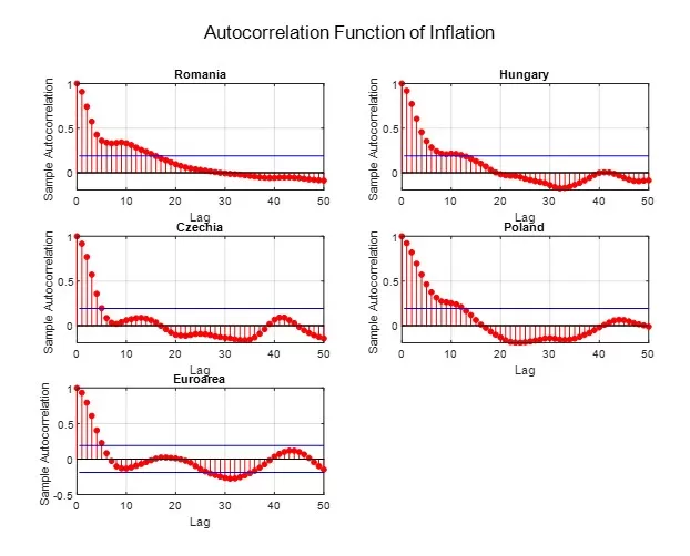
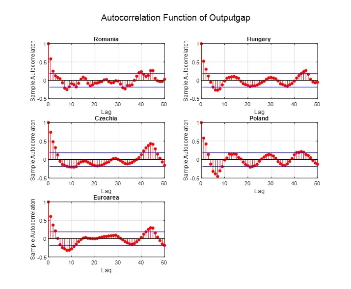
Another significant finding within the behavioral model framework is the presence of serial correlation in both the inflation rate and the output gap, as evidenced by visual inspection of the two variables. Specifically, the inflation rate exhibits a first-order autocorrelation coefficient for all states between 0.90 and 0.93, while the output gap displays an autocorrelation coefficient between 0.52 and 0.73 (and without pandemic period between 0.60 and 0.90). This inertia, endogenously generated within the behavioral model, represents a crucial characteristic observed in the empirical data, as depicted in Figures 7 and 8.
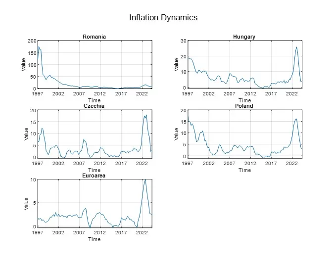
Figure 7: Inflation dynamics
Figure 8: Autocorrelation function of inflation
Figure 9: Autocorrelation function of output gap
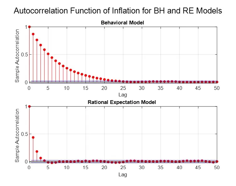
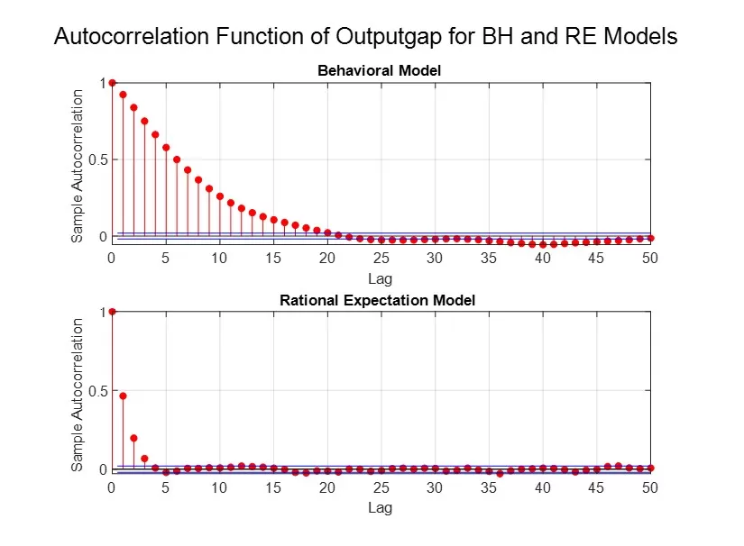
As mentioned earlier, the behavioral model can generate this inertia endogenously, mimicking the dynamics of the observed variables of interest, in contrast to the results obtained through the NK model with rational expectations, which is presented in Figures 10 and 11.Figure 10: Autocorrelation function of inflation in Behavioral Model vs Rational Expectation Model
Figure 11: Autocorrelation function of output gap in Behavioral Model vs Rational Expectation Model
In Figures 7 and 8, we present the evolution of the annual inflation rate in the selected states for the period 1997Q1-2024Q2, as well as the autocorrelation functions of these variables. In Figure 9, we show the autocorrelation functions of the output gap. As can be observed visually, there is a high degree of autocorrelation in the empirically observed variables, which persists for a long period—approximately six quarters in the case of the Eurozone and Czechia, and up to around 15-20 quarters for Romania, Hungary, and Poland, for inflation, while for the output gap, a similar pattern is observed across all countries, with persistence lasting around 3-4 quarters.
To assess the extent to which the key variables (inflation and the output gap) simulated within the two models—the behavioral model and the rational expectations model—exhibit these characteristics, we analyze their respective autocorrelation functions. Figures 10 and 11 demonstrate that the variables simulated by the rational expectations model exhibit a low degree of autocorrelation, even when structural inertia is incorporated into the model, as outlined in Section II.2. In contrast, the behavioral model succeeds in producing key variables that display a higher and more persistent degree of autocorrelation, both in the case of inflation (with a first-order autocorrelation of 0.8 and persistence lasting up to 20 quarters) and in the case of the output gap (with a first-order autocorrelation of 0.9 and persistence of up to 15 quarters).
As shown by De Grauwe (2019), the explanation for these results lies in the mechanism of expectation formation:
The equations above demonstrate that market expectations are represented by the proportion of agents using the extrapolation rule to forecast the output gap and inflation. This introduces serial correlation of the two variables into the model, with the degree of correlation depending on the proportion of agents using the extrapolation rule. As mentioned earlier, the selection of the rule is conditioned by its performance in forecasting the variable of interest. Additionally, these expectations have a self-fulfilling property: high performance of the output gap extrapolation rule will generate excess aggregate demand, leading to a continued increase in the rule’s performance.
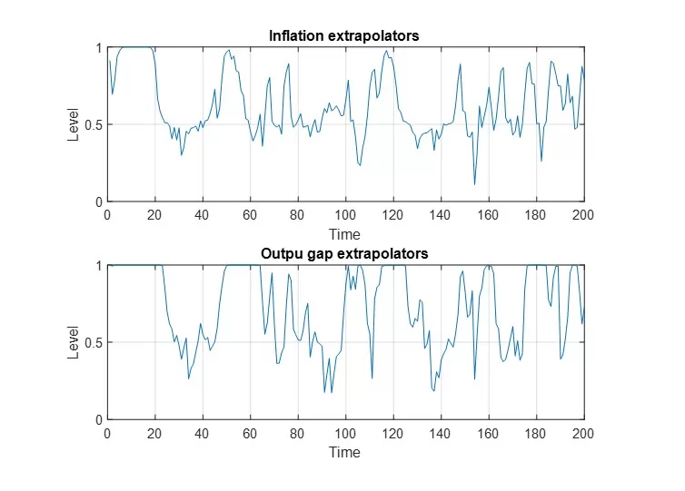
Figure 12: Proportion of agents using the extrapolation rule – inflation and output gap
Figure 12 presents the proportions of agents using the extrapolation rule for forecasting inflation and the output gap. It is observed that, for most of the time, the share of extrapolating agents exceeds 50%, sometimes reaching as high as 100%. The results indicate an average proportion of 65% for inflation and 75% for the output gap. This suggests that the extrapolation rule generally has a relatively superior performance. Furthermore, the variability of these probabilities over time highlights that agents adjust their forecasting rules based on the rule’s performance.
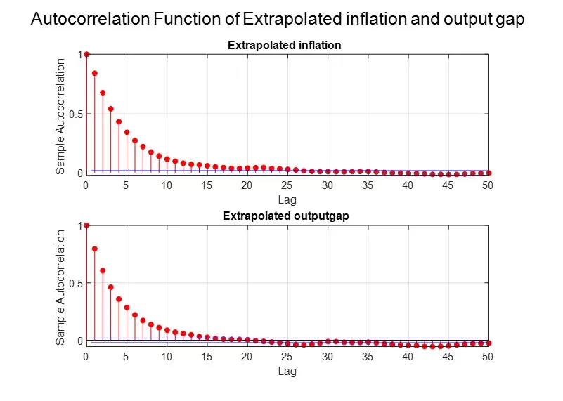
Figure 13: ACF of extrapolated inflation and ACF of extrapolated output gap
Figure 13 presents the autocorrelation functions (ACF) of extrapolated inflation and the output gap. It is observed that the degree of serial correlation for both variables is high, a characteristic closely related to the self-fulfilling nature of expectations: upon observing a positive output gap in the previous period, agents will extrapolate a positive value for the subsequent period, thereby reinforcing the economic boom (or recession)[9]. The results suggest that the expectation formation mechanism specified in the behavioral model is responsible for generating the serial correlation of inflation and the output gap.
In contrast to the rational expectations model[10], the behavioral model endogenously produces this inertia because of the agents’ expectation formation process. The reasoning behind these results, as shown by De Grauwe (2019), is that a variable proportion of economic agents extrapolates either a positive or negative trajectory for the output gap and inflation based on the relative performance of the extrapolation rule; agents base their expectations on prior experiences. They do not change their expectation formation process in every period, exhibiting a certain degree of inertia. The process of switching forecasting rules is relatively slow and occurs after accumulating sufficient evidence that the alternative rule has superior performance.
Conclusions
The main results obtained within the Neo-Keynesian behavioral model lead to the conclusion that the introduction of the limited rationality hypothesis for economic agents generates a macroeconomic dynamic that better captures the observed evolution of the inflation rate and the output gap. We have shown that, in the behavioral model presented, economic agents use two simple rules (heuristics) to form inflation and output gap expectations, which they periodically evaluate based on a success criterion. Thus, they employ a trial-and-error learning strategy, avoiding repeated mistakes. At the same time, the existence of these two rules implies heterogeneity within the model and enables interaction between economic agents, who can influence each other.
The two rules are the fundamentalist rule, where agents forecast the equilibrium value of the output gap and the inflation target, and the extrapolation rule, where agents’ expectations are based on previous values of the forecasted variable. This expectation formation mechanism allows for the introduction of an animal spirit variable, representing an index that quantifies market sentiment, which fluctuates between periods of generalized optimism or pessimism.
The animal spirit variable plays a crucial role in the model, leading to the main results analyzed, namely the non-normal distribution of the output gap and the presence of a high degree of autocorrelation in both inflation and the output gap.
Consistent with the characteristics of observed real data, the behavioral model generates an output gap that does not follow a normal distribution. This non-normality reflects the cyclical nature of economic activity. The animal spirit variable shows a distribution with concentrations at its extremes, which explains the presence of periods of generalized market optimism and pessimism. Additionally, a high correlation between the output gap and animal spirit is observed, explained by the self-fulfilling nature of expectations: agents’ sentiment influences the cyclical position of the economy, which, in turn, impacts economic sentiment. Thus, the leptokurtic distribution of the output gap produced by the behavioral model stems from the distribution of the animal spirit, with market sentiment variability endogenously generating periods of boom and recession typical of economic activity dynamics.
The second important result obtained in the behavioral model is the presence of serial correlation in both the inflation rate and the output gap. Comparing the results of the behavioral model with those of the classic model, we observe that the former is capable of endogenously producing inertia similar to that present in real data, without the need to introduce the assumption of serial correlation of errors. This result is driven by the expectation formation mechanism, through which serial correlation is introduced into the model, with its degree depending on the proportion of agents using the extrapolation rule, selected based on its performance. Since expectations have the self-fulfilling property, a high performance of the output gap extrapolation rule will generate excess aggregate demand, enhancing the performance of this rule and implicitly increasing the proportion of agents using it.
We can thus conclude that by incorporating hypotheses related to the way economic agents form their expectations, within the context of limited rationality, a macroeconomic dynamic is obtained that better reflects the observed dynamics of the output gap and the inflation rate. The further development of behavioral models lays the groundwork for improving the analytical framework of interactions between key macroeconomic variables.
References
Blattner, T.S., & Margaritov, E. (2010). Towards a Robust Monetary Policy Rule for the Euro Area. ECB Working Paper No. 1210.
Brock, W.A., & Hommes, C.H. (1997). A Rational Route to Randomness. Econometrica, 65(5), pp. 1059-1095.
Curtin, R. (2019). Consumer Expectations: Micro Foundations and Macro Impact. Cambridge: Cambridge University Press.
De Grauwe, P. (2011). Animal Spirits and Monetary Policy. Economic Theory, 47(2-3), pp. 423-457.
De Grauwe, P. (2012). Lectures on Behavioral Macroeconomics. Princeton, NJ: Princeton University Press.
De Grauwe, P. (2012). Lectures on Behavioral Macroeconomics. Princeton, NJ: Princeton University Press.
De Grauwe, P., & Ji, Y. (2019). Behavioural Macroeconomics: Theory and Policy. Oxford: Oxford University Press.
De Grauwe, P., & Macchiarelli, C. (2015). Animal Spirits and Credit Cycles. Journal of Economic Dynamics and Control, 59, pp. 95-117.
De Grauwe, P., & Ji, Y. (2018). Behavioural Economics is Useful Also in Macroeconomics: The Role of Animal Spirits. Comparative Economic Studies. ISSN 0888-7233.
DellaVigna, S. (2009). Psychology and Economics: Evidence from the Field. Journal of Economic Literature, 47(2), pp. 315-372.
Frederick, S., Loewenstein, G., & O’Donoghue, T. (2002). Time Discounting and Time Preference: A Critical Review. Journal of Economic Literature, 40, pp. 351-401.
Gali, J. (2008). Monetary Policy, Inflation, and the Business Cycle. Princeton, NJ: Princeton University Press.
Jang, T.S., & Sacht, S. (2016). Animal Spirits and the Business Cycle: Empirical Evidence from Moment Matching. Seoul National University; Kiel University and Kiel Institute for the World Economy.
Kahneman, D. (2003). Maps of Bounded Rationality: Psychology for Behavioral Economics. The American Economic Review, 93(5), pp. 1449-1475.
Kahneman, D., & Tversky, A. (1979). Prospect Theory: An Analysis of Decision Under Risk. Econometrica, 47(2), pp. 263-291.
Kahneman, D., & Tversky, A. (1974). Judgment Under Uncertainty: Heuristics and Biases. Science, 185(4157), pp. 1124-1131.
Loewenstein, G., & Prelec, D. (1992). Anomalies in Intertemporal Choice: Evidence and an Interpretation. The Quarterly Journal of Economics, 107(2), pp. 573-597.
Rabin, M. (2002). A Perspective on Psychology and Economics. European Economic Review, 46(4-5), pp. 657-685.
Thaler, R.H. (1981). Some Empirical Evidence on Dynamic Inconsistency. Economics Letters, 8(3), pp. 201-207.
Weber, R., & Dawes, R. (2005). Behavioral Economics. In: Smelser, N.J., & Swedberg, R. (Eds.), The Handbook of Economic Sociology. Princeton University Press, pp. 90-108.
[1] Paul De Grauwe și Yuemei Ji, 2019, Behavioural macroeconomics, Theory and Policy. Oxford University Press.
[2] Brock and Hommes (1997, 1998)
[3] Kahneman (2002).
[4] This approach is commonly used in the specialized literature on discrete choice theory.
[5] The proportion of agents extrapolating a positive output gap is given by .
[6]The proportion of agents anticipating a zero output gap is given by .