Walquer Huacani1, Nelson P. Meza2, Franklin Aguirre3, Darío D. Sanchez4 y Evelyn N. Luque5
1,2,3,4 Professional Academic School of Mining Engineering, Micaela Bastidas National University of Apurímac
5 Professional School of Computer Engineering and Systems, Micaela Bastidas National University of ApurímacAbancay, Apurímac, Perú
Volume 2022,
Article ID 988227,
Journal of Internet and e-business Studies,
14 pages,
DOI: 10.5171/2022.988227
Received date: 26 April 2021; Accepted date: 16 September 2021; Published date: 7 January 2022
Academic Editor: Leticia del Pilar Campos Olivares
Cite this Article as:
Walquer Huacani, Nelson P. Meza, Franklin Aguirre, Darío D. Sanchez y Evelyn N. Luque (2022)," Analysis of Deforested Area Using Google Earth Engine in The Period 2001-2020 In the Apurimac Region", Journal of Internet and e-Business Studies, Vol. 2022 (2022), Article ID 988227, DOI: 10.5171/2022.988227
The objective of this study is to analyze the deforestation of forest cover in the Apurimac region between 2001 and 2020 using the Google Earth Engine (GEE) platform, a planetary-scale platform for the analysis of environmental data. The methodology used in the analysis of the deforested area is based on the classification of cover, using a supervised classification method developed by the University of Maryland, based on a “decision tree”. For the characterization of the extent and change in coverage, the band channels of Landsat 7 and 8 satellite images were processed, respectively. For the processing, the updated data of the gross forest cover loss for the years 2001-2020 were used, making use of raster information, within the (GEE) platform. For the statistical treatment, descriptive statistics were applied to analyze the variables and establish if there is a correlation. The results of the study determined that there is a total deforested area of 3958.231 ha, with an annual rate of 109.15% for the year 2017 and with a negative annual rate of -67.05% for the year 2018, during the study period. It is concluded that in the descriptive statistics, the -p-value (bilateral) of significance is 0.81, which is greater than (0.05), then it is stated that there is no significant relationship between the variable’s deforestation and the years.
Keywords: Forest cover, deforestation, Google Earth Engine and Landsat
Introduction
During the dry season, weeds are burned, and in many cases, fire spreads, destroying the forest and causing damage to the vegetation. The total area of forests in the world is 4.06 billion hectares (ha), corresponding to 31 percent of the total land area. This area is equivalent to 0.52 ha per person (FRA, 2020). An estimated 420 million ha of forest have been lost worldwide to deforestation since 1990 however, the rate of forest loss has decreased considerably. In the last five-year period (2015-2020), the annual rate of deforestation was estimated at 10 million ha, down from 12 million ha in 2010-2015 (FAO, 2020).
Peru is a country with 60% forest cover, 94% of which is in the Amazon region. Forests play an important role in national debates about the fate of the Peruvian Amazon and whether to promote conservation, economic growth and development, or a balance between them (Menton and Cronkleton, 2019). Recently, the concern for biodiversity conservation and climate change mitigation has led to policies promoting reduced deforestation (e.g., participation in REDD+ (Reducing Emissions from Deforestation and Degradation) initiatives; and the National Forest and Climate Change Strategy (MINAM, 2016)). At the same time, other policies have created incentives for the agricultural expansion that lead to deforestation. For 2017, deforestation in the Peruvian Amazon was reported at 143 000 ha (Finer & Novoa, 2018).
The Apurimac region has a primary natural forest of 57 438 ha, (Kometter, 2018). Primary forests are composed of native species in which there are no evident signs of human activities and where ecological processes have not been significantly altered. Forests are the reservoir of carbon which is found in living biomass (44%) and in soil organic matter (45%), while the rest is in dead wood and litter (FRA, 2020), due to degradation; and forest fires, logging all by human action, The Andean Forests Program (PBA) is a regional initiative of the Global Climate Change Program (GCCP) of the Swiss Agency for Development and Cooperation (COSUDE), which contributes others the Andean population living around the Andean forests to reduce their vulnerability to climate change and receive social, economic and environmental benefits from the conservation of Andean forests. A pilot area for forest restoration is being established, with the aim of improving the provision of ecosystem services, mainly water. To this end, the community delimited and fenced off the area to be restored, establishing the baseline, with studies on flora and fauna, soils, as well as livelihoods and knowledge. Based on this information, the orientation and the approach that the community itself has decided to give to the restoration, the Forest Restoration Plan has been collaboratively developed in several communities in the Apurimac Region (Kometter, 2018).
Forest cover plays a critical role in providing important ecosystem services, including biodiversity richness, climate regulation, carbon storage and water supply (Foley et al., 2005) However, detailed spatial and temporal information on global-scale forest cover change at high resolution did not exist until M.C. Hansen and his team at the University of Maryland, USA, developed a global-scale forest change work and published it in 2013 (Hansen et al., 2013), where they mapped the extent, loss and gain of global tree cover that they update annually, from the period 2000 to 2020 from Landsat imagery at 30 spatial resolution, for time series analysis (Hansen et al.,2013).
On the other hand, deforestation and forest degradation are among the main causes of biodiversity loss, increased carbon emissions and other greenhouse gases (GHG) ((Nguyen et al., 2021); Sasaki et al., 2011; Budiharta et al., 2014). However, in recent years, while deforestation rates have been reduced in many countries, forest degradation has increased (Budiharta et al., 2014).
Forest deforestation monitoring, using Landsat images, has already been reported (Broich et al., 2011; Killeen and Calderon 2007; Potapov et al., 2015). The main limitation for the analysis with images obtained from optical sensors is the presence of cloud cover. This problem has also been overcome by using cloudiness filters in Landsat scenes (TOA). The methodology for processing Landsat- ETM+ scenes obtained between 2001 and 2020 for the Apurimac region used images of bands 3, 4, 5, 7, the Normalized Difference Vegetation Index (NDVI), Normalized Band Ratio (NBR) and more than 500 metrics or statistical variables created using the aforementioned bands. This land cover’s classification was performed using a supervised classification method developed by the University of Maryland and is based on a “decision tree”. The classification algorithm uses only two types of samples (Forest/Non-forest or Loss/Non-loss). These training samples for determining deforested areas, were performed on the Google Earth Engine (GEE) platform, which is composed of four main elements. The first is Google’s infrastructure, which makes its servers available to the user, allowing parallel analysis with about 10,000 CPUs. This speeds up the processing speed, compared to an individual computer (Moore, 2017). The second element is the data pool (datasets). Google has stored all the images from various sensors (Landsat, Sentinel and MODIS, among others). These databases are updated as new images are taken (about 6000 new scenes per day), thus creating a huge catalog of geospatial data. These databases can be queried through different criteria (quality, location, dates) without the need to download or request access to the images (Gorelick et al., 2017).
The third element is the API (Application Program Interface), which consists of a series of pre-established commands and functions, written in JAVA language, which allows easy programming when developing algorithms for research. Finally, the fourth element is the Code Editor, which is an integrated online development environment, where all the elements come together. This is where the user can, through working code (“scripts”), call the data, process it and visualize it virtually with Google’s servers, thus having their results and information in the cloud.
This paper presents an analysis of forest degradation based on the results of time series analysis of Landsat images from forest change data obtained from Hansen and his team at the University of Maryland, USA, developed on the GEE platform during the period 2001-2020.
Theoretical framework
Forest degradation
Forest degradation has been defined as a process of reduction in forest quality (Lund, 2009). It is also considered as a process of change that negatively affects forest characteristics (Simula, 2009). On the other hand, forest degradation refers to a loss of carbon stocks within forested areas that remain forested. It is a negative impact caused by humans that can affect the ecological processes of ecosystems (Herold et al., 2011).
Definitions of forests and deforestation
FAO defines forest as an area with trees over 5 meters high and with a canopy cover of more than 10%, in areas of more than 0.5 hectares. This definition does not include areas that are for agricultural or urban use, but does include plantations used for forestry or protection purposes, protected areas and areas of scientific, historical or cultural interest (FAO, 2001). On the other hand, the United Nations Framework Convention on Climate Change (UNFCCC or UNFCCC) defines forest as a minimum land area of 0.05-1.0 hectares with tree canopy cover of more than 10% to 30%, with a minimum height of 2-5 meters.
Motor Google Earth Engine (GEE)
Google Earth Engine (GEE) is a planetary-scale platform for environmental data analysis. It brings together more than 40 years of current and historical satellite imagery from around the world, and provides the tools and computational power needed to analyze and extract information from this huge store of data. Among one of its applications is land cover change detection (Google, 2016). GEE is a massively parallel technology for high-performance processing of geospatial data, and hosts a copy of the entire catalog of Landsat and other imagery (Venturino et al., 2014).
Landsat TOA images
Landsat 8 Collection 1 Tier 1 composite is made from orthorectified Tier 1 scene using computed top-of-atmosphere (TOA) reflectance (Chander et al., 2009). These composites are created from all scenes in each 8-day period starting from the first day of the year and continuing through the 360th day of the year. The last composite of the year, starting on day 361, will overlap the first composite of the following year by 3 days. All images from each 8-day period are included in the composite, with the most recent pixel as the composite value.
Materials and Methodology
Study Area
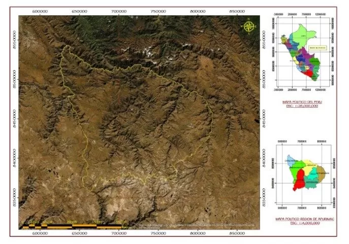
The study area is the Apurímac region (Fig 1), located in the Andean region of Peru, with a surface area of approximately 21 113.19 km2. The natural vegetation includes a diversity of categories, ranging from high Andean grasslands, natural and planted forests, to a series of scrub associations. However, the dominance of grasslands (45% of the departmental extension) is notorious and is found mainly in the highlands in the south of the department, in the provinces of Aymaraes, Antabamba, Grau and Cotabambas.
Figure 1: Geographical location of the Apurimac region
Note. Prepared by the author based on the information analyzed
The relief is characterized by the presence of mountain ranges, whose altitudinal differences make up a gradient that ranges from 1,000 masl in the Apurimac River canyon, as the lowest point, to the highest point at 5,450 masl in the snow-capped mountains of Ampay, in the province of Abancay. Sixty-six percent of the territory has steep to steep slopes, while only 33% corresponds to flat to moderately steep categories.
Materials
This study is based on data from the 2013 Global Forest Change research. This work is the result of the analysis over time, of 654178 Landsat images, which were resampled, radiometrically corrected and filtered (presence of clouds) to generate different time series metrics, which were used to classify the images with a decision tree algorithm. According to the authors’ evaluation, the database is reliable. For example, the class “forest loss” presents omission and commission errors of (13%) of forest extent and its changes, in the period from years 2000 to 2012 for the period 2000 to 2020 (Hansen et al., 2013). Information about these results can be obtained from the page: http://earthenginepartners.appspot.com/science-2013-global-forest. To corroborate their data, Hansen’s study compared them with those of the Global Forest Resources Assessments (FRA, 2020). A project of the Food and Agriculture Organization of the United Nations (FAO, 2020), being a global standard reference for forest resources. Although for many global regions there are discrepancies with FRA results the region with the highest correlation between both methodologies is in Latin America (Hansen et al., 2013). Two techniques were used to validate the cover change, loss or gain data: the first using a stratified random sampling of 120 blocks per a specific biome; the second using data from NASA’s GLAS (Geoscience Laser Altimetry System) LiDAR (Light Detection and Ranging) system (Hansen et al., 2013).
Methodology
Today, there is a diversity of techniques to analyze deforestation, such as: change detection, map algebra, change matrix, multitemporal analysis, and digital processing of satellite images, among others (Hansen et al., 2013); Potapov et al., 2015). Likewise, to investigate the deforestation processes that drive the loss of forest cover, studies have been conducted using exploratory data analysis techniques, regressions, Bayesian statistics, and neural networks (Monjardin et at., 2017). Today, with the advancement of technology RStudio and the Google Earth Engine platform are applied.
The methodology used for the training work is from the results of time series analysis of Landsat images in the characterization of the extent and change of the global forest from 2000 to 2020 (Hansen et al., 2013). To develop this mapping, 654 178 Landsat images were analyzed, which were resampled, radiometrically corrected and filtered (presence of clouds) to generate different time series metrics, which served to classify the images with a decision tree algorithm (Perilla & Mas, 2020). These images go through a preprocessing, where they are calibrated to reflectance values at the top of the atmosphere (TOA) and normalized to obtain images with homogeneous reflectance values. They are available at:
https://developers.google.com/earthengine/datasets/catalog/UMD_hansen_global_forest_change_2020_v1_8. To download the individual 10×10 degree granules defined as a stand replacement disturbance or a change from forest to non-forest state, coded as 0 (no loss) or as a value in the range 1-20, representing the detected loss of the map region, one can find them available at the URLs: https://storage.googleapis.com/earthenginepartners-hansen/GFC-2020-v1.8/Hansen_GFC-2020-v1.8_lossyear_40N_080W.tif.
Geometric corrections
These composite reference images are median observations from a set of growing season observations evaluated for quality in four spectral bands, specifically Landsat bands 3, 4, 5 and 7. These are characterized by being geometrically rectified and free of sensor-related distortions.
Calibration and data normalization
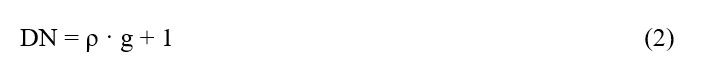
The digital levels (ND) of the raw images were calibrated to top-of-atmosphere (TOA) reflectance values. Correction was performed using the approach described by (Chander et al., 2009), with coefficients taken from the metadata. First the conversion to radiance values was made using the following equation:
Where:
Pλ = Reflectance at the top of the atmosphere.
π = Lambertian target hypothesis .
Lλ = Total radiance measured by the satellite.
d2 = Earth-Sun distance in astronomical units, and d is calculated as:
d = 1- 0,0167 cos (2π (Julian day-3)/365).
ESUNλ = Spectral solar irradiance at peak.
Cos ϴs = Cosine of the solar zenith angle.
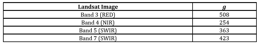
Output data
For data output and to facilitate the processing of the metrics, the normalized reflectance data were reduced to 8 bits using a
scale factor (g). This factor was assigned for each band in order to maintain the dynamic range of each band.
According to (Hansen et al., 2013) the factor (g) was chosen independently for each band to preserve the band-specific dynamic range, as shown in the following Table 1:
Table 1: Landsat scaling factors (g)
Creation of Metrics
The time series analysis of Landsat ETM images uses the multitemporal metrics (DeFries 1995; Hansen et al., 2008; Potapov et al., 2015), which allow the accurate detection of change over 20 years of observations. The dataset used for the metrics was stored in quadrats of 2000 pixels per side. Thus, 458 quadrats were obtained for the total area of the country containing all the metrics that were used for classification. Trees are defined as vegetation over 5 m tall and with canopy cover greater than 10%, in areas larger than 0.5 hectare, (FAO, 2020) and are expressed as a percentage per output grid cell as “2000% tree cover”. “Forest cover loss” is defined as a stand replacement disturbance, or a change from forest to non-forest status, during the period 2000-2020. Forest cover gain” is defined as the inverse of loss, or a change from non-forest to forest entirely within the period 2000-2012. “Forest Loss Year” is a disaggregation of total “Forest Loss” into annual time scales (Hansen et al., 2013).
Classification Process
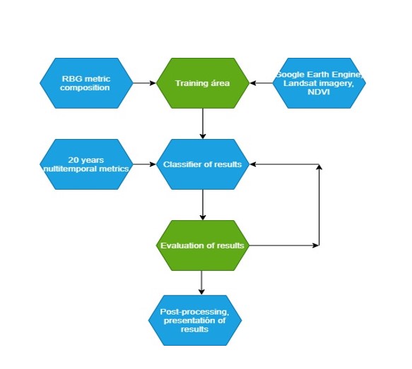
The supervised classification algorithm was developed by the University of Maryland and is a method based on a “decision tree” that is generated from manually created samples, by interpreting patterns visually for the classes to be classified. In this case, it is the Forest and Non-forest class generated from the metric compositions in RGB color and using information from available satellite sensor images (Landsat 7, Landsat 8). The classification workflow is shown in Figure 3.
Figure 3. Forest cover loss classification process workflow
Note. Prepared by the author based on the information analyzed
Analysis of spatial variation
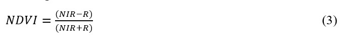
Among the main remote sensing techniques applied to satellite image processing for the analysis of vegetation dynamics, the Normalized Difference Vegetation Index or NDVI stands out (Georganos et al., 2017; Tian et al., 2015; Zhao et al., 2015; Fonseca, 2000).
For the analysis of the NDVI vegetation index, one can resort to the NIR and RED working bands to compose the normalized index and quantify the vegetation values. The available bands are outlined under the beginning and end of the historical period, so one can obtain NDVI values per year and access each of the collections at: Hansen / UMD / Google / USGS / NASA.
The Normalized Difference Vegetation Index (NDVI) is a numerical indicator using the red and near-infrared spectral bands. NDVI is highly associated with the vegetation content. Higher NDVI values correspond to areas that reflect more in the near-infrared spectrum.
Higher near-infrared reflectance corresponds to denser and healthier vegetation.
This method is used for mapping vegetation index surfaces. The band algebra is as follows:
Where NIR is the high reflectivity in the near infrared, and R is the reflectivity in the red.
Extraction and visualization of deforestation
There are many methods to extract and visualize the remote sensing dataset. For example, using the Google Earth Engine JavaScript API, one can analyze the results directly, using the asset ID UMD / hansen / global_forest_change_2029_v1_8., generating the indices from annual Landsat composites and the calculation of tree loss per year for the regions of interest (Hansen et al., 2013). However, it is also performed in QGIS. First, it is necessary to install the Google Earth Engine plug-in, in the Python console and the global forest cover data will appear running the script. On the other hand, it can be determined with R, which is a working environment for running statistical analysis and creating graphs (R Development, 2011).
Processing of results in Google Earth Engine (GEE)
For the present study of cover loss, the Google Earth Engine (GEE) platform was used with raster information obtained from the page: https://developers.google.com/earth engine/datasets/catalog/UMD_hansen_global_forest_change_2020_v1_8. Data from the provider can be found in: Hansen/UMD/Google/USGS/NASA. For the statistical analysis, the R programming language was used.
For the generation of annual forest cover map, the Google Earth Engine (GEE) platform was used, and Landsat image scenes were also used. Using the Web-based code editor for JavaScript API performing filters to the collection of entities, this planetary scale platform for environmental data analysis, gathers more than 40 years of current and historical satellite images from around the world, and offers the tools and computational power needed to analyze and extract information from this huge data warehouse. Among one of its applications is land cover change detection (Google, 2016). The results of annual forest cover degradation in the Apurimac region can be visualized by accessing the following GEE link:
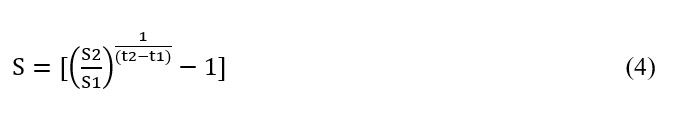
The mathematical formula is most commonly used to calculate the annual rate of change of deforestation, in such a way that allows the comparison of results from different periods. The equation corresponds to the one used by (FAO, 1996).
Where:
S: Exchange rates for different years
S1: Area at the beginning of the period
S2: Area at the end of the period
t2: Starting year of the period
t1: Ending year of the period
Results
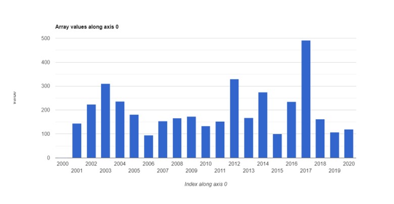
For the deforested area count for different periods (2001-2020), for the Apurimac region, using raster information, where the data comes at a global level within the GEE platform, the results of the deforestation of the forest cover determine a loss of 3958.231 ha, as shown in Figure 4.
Analysis of results
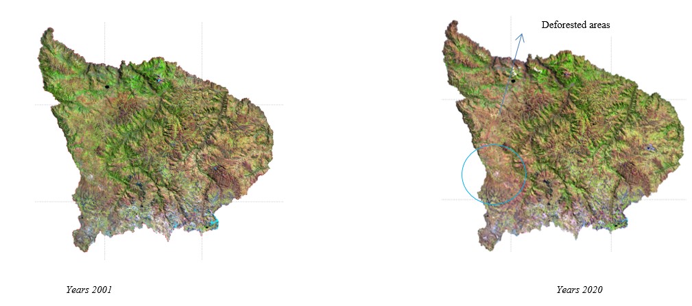
As can be seen from Fig. 6, shows the processing of the image data obtained from Global Forest Change 2001-2020, where the most degraded areas are the sectors of Chincheros, Uripa, Occobamba and Cocharas.
Figure 4. Deforestation of the Apurimac region for the years (2001 – 2020)
Note. Prepared by the author based on the information analyzed
Forest degradation continues to advance at an alarming rate, contributing significantly to the ongoing loss of biodiversity. Since 1990, an estimated 420 million hectares of forest have been lost to land-use change, even though the rate of deforestation has declined over the past three decades. Between 2015 and 2020, the deforestation rate was estimated at 10 million hectares per year, while in the 1990, it was 16 million hectares per year (FRA, 2020).
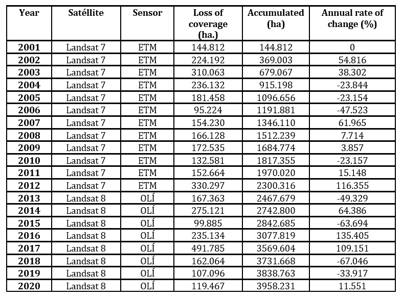
According to Table 4, it is visualized that, in the years 2003, 2012, and 2017, deforestation rates were the highest, reaching a maximum value of 491.785 ha. While for the period 2017 and year 2006 deforestation reached a minimum value of 95.224 ha.
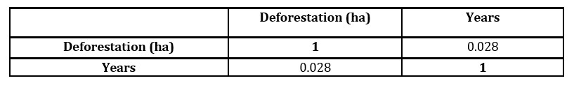
Table 2: Correlation coefficient of deforestation period 2001-2020
The results of table 2 of correlation r= 0.028; of deforestation in the period 2001-2020, show that there is a very weak positive trend. Therefore, the mean is an unreliable representative index, so there is no relationship between these variables.
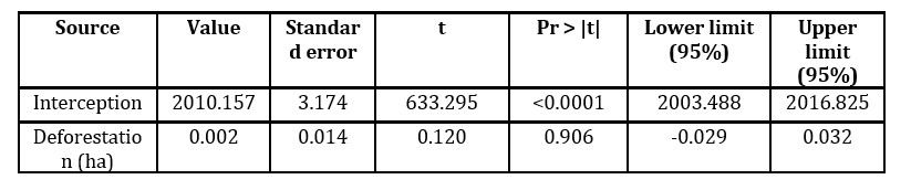
Table 3: Deforestation model parameters for the period (2001-2020)
The Pvalue of significance is 0.906, which is greater than (0.05), so it is affirmed that there is no significant relationship between the variables deforestation and the period (years).
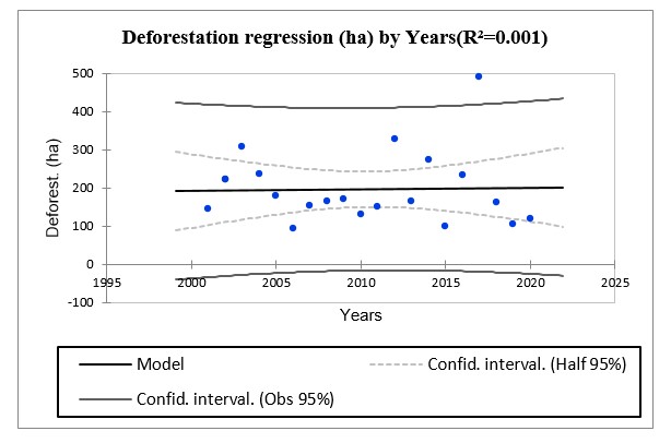
Figure 5: The linear regression of deforestation with respect to years, where the equation shows a very weak positive correlation (+), with a quadratic correlation coefficient R2= 0.001, indicating that the explanatory variable (years) represents 0.10%, which is the percentage of variability with the dependent variable (deforestation)
Results of deforested areas
Table 4: Deforested areas in the period 2001 – 2020
In Table 4; shows the deforested areas of the province of Abancay, for a period of 20 years. Approximately 3 958.231 ha haves been lost. In the year 2001, it was reduced by 144.812 ha; however, the years 2003, 2012 and 2017, witnessed the highest amount of loss of deforested areas. On the other hand, in the year 2020, 119.467 ha haves been deforested. Deforestation rates vary for different years, for example, for the year 2017, it was 109.151%.
Figure 6. Combination of Landsat image bands (RGB) for the years 2001, 2020
Note. Prepared by the author based on the information analyzed
As a result of this analysis, the most deforested areas are the Chincheros, Uripa, Occobamba and Cocharas sectors, as shown in Figure 6.
Conclusions
In this research, the loss of deforested primary forest cover was determined on the Google Earth Engine platform for the period 2001-2020 in the Apurimac region.
According to the analysis, the deforested areas in the Apurimac region in a period of 20 years are 3958,231 ha, with an annual rate of change of 109,151% for the year 2017, and with a negative annual rate of -67.046% for the year 2018.
In the statistical analysis, it can be stated that there is a correlation level r2= 0.001; of deforestation in the period 2001-2020. It is observed that there is a very weak positive trend, therefore the mean is an unreliable representative index and so, there is no relationship between the variables.
In the statistical conclusion, the -p (bilateral) significance value is greater than (0.05), so it is determined that there is no significant relationship between the variables deforestation and the period (years).
The most important contributions of this study lie in developing standards for the rational use of forest resources, implementing strategies to combat deforestation, and encouraging the planting of one tree per person.
Broich, M., M. C. Hansen, F. Stolle, P.V. Potapov, B.A. Margono y B. Adusei 2011 Remotely sensed forest cover loss shows high spatial and temporal variation across Sumatera and Kalimantan, Indonesia 2000-2008. Environmental Research Letters, 6/1, doi:10.1088/1748-9326/6/1/014010.
Budiharta S, Meijaard E, Erskine PD, et al., (2014) Restoring degraded tropical forests for carbon and. Available at: https://iopscience.iop.org/article/10.1088/1748-9326/9/11/114020/pd
Chander, G., Markhan, B., Helder, D., (2009) Summary of current radiometric calibration coefficients for Landsat MSS, TM, ETM+, and EO-1 ALI sensors May 2009. Remote Sensing of Environment 113(5):893-903 DOI: 10.1016/j.rse.2009.01.007
United Nations Framework Convention on Climate Chang (UNFCCC, 1992)
DeFries, R., Hansen, M., and Townshend, J. (1995). Global discrimination of land cover types from metrics derived from AVHRR Pathfinder data. Remote Sens. Environ. 54 209-22.
Global Forest Resources Assessment, FRA (2020) Main findings. FAO. 2020. https://doi.org/10.4060/ca9825en
FAO (Food and Agriculture Organization of the United Nations). 1996. Forest resources assessment 1990. Survey of tropical forest cover and study of change processes. 154 p.
Fonseca, E. L. 2000 Caracterizacao espectral e índice de vegetacao em Paspalum Notatum Flügge vas. Notatum com visitas a modelagem de crescimento (Dissertacao de Mestrado). Porto Alegre: Pós-graduacao em Fitotecnia – Universidade Federal do Rio Grande do Sul. forests for carbon and biodiversity. Environ Res Lett. doi: 10.1088/17489326/9/11/114020
Georganos, S., Abdulhakim, A., Tenenbaum, D., & Kalogirou, S. 2017 “Examining the NDVI – rainfall relationship in the semi-arid Sahel using geographically weigted regression”. Journal of Arid Environments, 64-74.
Gorelick, N., Hancher, M., Dixon, M., Ilyushchenko, S., Thau, D., & Moore, R. (2017). Google Earth Engine: Planetary-scale geospatial analysis for everyone. Remote Sensing of Environment, 202, 18-27. https://doi.org/10.1016/j.rse.2017.06.031
Hansen, M. C., Roy, D., Lindquist, E., Justice, C. O., and Altstaat, A. (2008). A method for integrating MODIS and Landsat data for systematic monitoring of forest cover and change in the Congo Basin. Remote Sens. Environ. 112 2495-513.
Hansen, M. C., P. V. Potapov, R. Moore, M. Hancher, S. A. Turubanova, A. Tyukavina, D. Thau, S. V. Stehman, S. J. Goetz, T. R. Loveland, A. Kommareddy, A. Egorov, L. Chini, C. O. Justice, and J. R. G. Townshend. 2013. “High-Resolution Global Maps of 21st-Century Forest Cover Change.” Science 342 (15 November): 850–53. Data available on-line from: http://earthenginepartners.appspot.com/science-2013-global-forest.
Herold M, Román-Cuesta R.M., Mollicone D, Hirata Y, Van Laake P, Asner G.P., Souza C, Skutsch M, Avitabile V, MacDicken K. (2011) Options for monitoring and estimating historical carbon emissions from forest degradation in the context of REDD+. Carbon Balan
Killeen, T. J., V. Calderon, L. Soria, B. Quezada, M. K. Steininger, G. Harper, L. A. Solorzano, y C. J. Tucker, 2007 Thirty years of land-cover change in Bolivia. Ambio, 36(7), 600-606.
Lund H. (2009) What is a degraded forest? White Paper on Forest Degradation Definitions Prepared for FAO.
C., P. V. Potapov, R. Moore, M. Hancher, S. A. Turubanova, A. Tyukavina, D. Thau, S. V. Stehman, S. J. Goetz, T. R. Loveland, A. Kommareddy, A. Egorov, L. Chini, C. O. Justice, and J. R. G. Townshend. 2013. “High-Resolution Global Maps of 21st-Century Forest Cover Change.” Science 342 (15 November): 850–53. Data available on-line from: http://earthenginepartners.appspot.com/science-2013-global-forest.
[MINAM] Ministry of Environment of Peru. 2016. National forest and climate change strategy. Supreme Decree 007- 2016-MINAM. Lima, Perú: MINAM.
Monjardín-Armenta, Sergio A., Pacheco-Angulo, Carlos E., Plata-Rocha, Wenseslao, & Corrales-Barraza, Gabriela. (2017). Deforestation and its causal factors in the state of Sinaloa, Mexico. Timber and forests, 23(1), 7-22. https://doi.org/10.21829/myb.2017.2311482
Moore, R. (Directora de Google Earth, Earth Engine y Earth Outreach). (2017). Accompanying presentation Earth Engine Users’ Summit 2017 (Videoconferencia). Recuperado de https://youtu.be/5yy1EwtZmhE
Perilla, G. y Mas, J. (2020). Google Earth Engine (GEE): A Powerful Tool Linking the Potential of Massive Data and the Efficiency of Cloud Processing DOI: doi.org/10.14350/rig.59929. Available at: www.investigacionesgeograficas.unam.mx
Potapov, P. V., Turubanova, S. A., Tyukavina, A., Krylov, A. M., McCarty, J. L., Radeloff, V. C., and Hansen, M. C. (2015).Eastern Europe’s forest cover dynamics from 1985 to 2012 quantified from the full Landsat archive. Remote Sens. Environ. 159 28-43.
R Development Core Team (2011) R: A Language and Environment for Statistical Computing. The R Foundation for Statistical Computing, Vienna, Austria. http://www.R-project.org/.
Sasaki N, Asner G, Knorr W, et al (2011a) Approaches to classifying and restoring degraded tropical forests for the anticipated REDD+ climate change mitigation mechanism. iForest – Biogeosciences For 4:1–6. doi: 10.3832/ifor0556-004
Simula M (2009). Towards a definition of forest degradation: Comparative analysis of existing definitions. Rome, Italy. 54p.
Tian, F., Fensholt, R., Verbesselt, J., Grogan, K., Horion, S., & Wang, Y. 2015 “Evaluating temporal cosistency of long-term global NDVI datasets for trend analysis”. Remote Sens, 326-340.
Venturino, R.; Schall, U. M.; Solichin, U. J. Google Earth Engine As a Remote Sensing Tool. International Journal of Remote Sensing & Geoscience, p. 1–15, 2014.
Zhao, Z., Goa, J., Wang, Y., Liu, J., & Li, S. 2015 “Exploring spatially variable relationships between NDVI and climate factors in a trasition zone using geographically weighted regression”. Appl. Climatol, 507-519.