Introduction
The confidence in Romanian economy can be a very exciting subject considering the way Romanians see the economic development and also from a foreign point of view. Also it is necessary to have a forecast of several indicators in order to invest in certain economic fields and Economic Sentiment Indicator (ESI) is one of them. But what is the way to do it if the calculated ESI is different from the real sentiment about the country economy? As presented in chapter 3, the ESI is calculated using five sector-specific confidence indicators. But is this calculus representative of the real sentiments about countries’ economies? The researchers think that the real confidences in economies are more nonlinear which can be determined with calculus. This is why Artificial Neural Networks are used to see if these types of methods can provide a better forecast than the simple calculus. The artificial neural networks have proved their effectiveness in simulating the nonlinear processes and phenomenon; moreover, they offer in almost all researches superiority over the other simulating methods.
The researchers knew that ANN can learn from the past ESI values, considering the five sector-specific confidence indicators, and they thought that the ANN will forecast accurate values of the ESI.
The data used for the all the trainings and simulations were taken from European Commission — Joint Research Centre website: http://composite-indicators.jrc.ec.europa.eu/CI_Econ0001.htm in January 2011.
The objectives of the research are as follows:
- Building, training and validating a specific ANN for the simulating of the Economic Sentiment Indicator considering five sector-specific confidence indicators and the imposed conditions;
- Testing the trained ANN in order to check that the difference between the real data and the simulated is smaller than 5%;
- Determining the trend of Economic Sentiment Indicator with the trained ANN;
- Establishing the sustainability of future ANN use for the forecast of the ESI.
Artificial Neural Network (ANN)
Today, Artificial Neural Network (ANN) can be found in the majority of the human life activity, their potential being considered immense. Starting with the human brain and continuing with the actual common application of the ANN, their use effectiveness is demonstrated as can be seen in Akira Hirose’s book “Complex-valued neural networks: theories and applications” [World Science Publishing Co Pte. Ltd, Singapore, 2003].
Regardless of the type, ANN has a few certain common unchallengeable elements mentioned by Zenon WASZCZYSZYN in his book: “Fundamentals of Artificial Neuronal Networks” [Institute of Computer Methods in Civil Engineering, 2000]:
- micro-structural components: processing elements — neurons or nodes
- input connections of the processing elements
- output connections of the processing elements
- the processing elements can have optional local memory
- transfer (activation) function, which characterizes the processing elements.
-
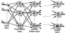
Figure 1. Schematic Representation of a Multilayer ANN
The schematic graphic representation of a multilayer ANN is presented in figure 1, were xi ( ) is the input ANN values, H1 and H2 are the numbers of neurons from the first and second hidden layer, M is the number of neurons from the output ANN layer and yj (
 ) is the values of the output data.
The Economic Sentiment Indicator (ESI)
The Economic Sentiment Indicator is used in order to combine business tendency surveys into a single cyclical composite or confidence indicator with a view to reduce the risk of false signals and provide a cyclical indicator with better forecasting and tracking qualities than any of its individual components, as defined by The European Commission
[http://ec.europa.eu/economy_finance/db_indicators/surveys/time_series/index_en.htm].
Economic Sentiment Indicator purpose is to track GDP growth at Member State, EU and euro-area level. The ESI can be viewed as a summary of the five sector-specific confidence indicators
[http://ec.europa.eu/economy_finance/db_indicators/surveys/documents/userguide_en.pdf].
- Industrial confidence indicator (INDU). The industrial confidence indicator is the arithmetic average of the balances (in percentage points) of the answers to the questions on production expectations, order books and stocks of finished products (the last with inverted sign). Balances are seasonally adjusted [http://ec.europa.eu/economy_finance/db_indicators/surveys/documents/userguide_en.pdf].
- Services confidence indicator (SERV). The services confidence indicator is the arithmetic average of the balances (in percentage points) of the answers to the questions on business climate and on recent and expected evolution of demand. Balances are seasonally adjusted.
- Consumer confidence indicator (CONS). The consumer confidence indicator is the arithmetic average of the balances (in percentage points) of the answers to the questions on the financial situation of households, the general economic situation, unemployment expectations (with inverted sign) and savings, all over the next 12 months. Balances are seasonally adjusted [http://ec.europa.eu/economy_finance/db_indicators/surveys/documents/userguide_en.pdf].
- Retail trade confidence indicator (RETA). The retail trade confidence indicator is the arithmetic average of the balances (in percentage points) of the answers to the questions on the present and future business situation and on stocks (the last with inverted sign). Balances are seasonally adjusted [http://ec.europa.eu/economy_finance/db_indicators/surveys/documents/userguide_en.pdf].
- Construction confidence indicator (BUIL). The construction confidence indicator is the arithmetic average of the balances (in percentage points) of the answers to the questions on order book and employment expectations. Balances are seasonally adjusted [http://ec.europa.eu/economy_finance/db_indicators/surveys/documents/userguide_en.pdf].
- Economic Sentiment Indicator purpose is to track GDP growth at Member State, EU and euro-area level. The ESI can be viewed as a summary of the five sector-specific confidence indicators.
The exact calculation of the ESI on the basis of its component series can be summarized by the following three simple steps
[http://ec.europa.eu/economy_finance/db_indicators/surveys/documents/userguide_en.pdf]:
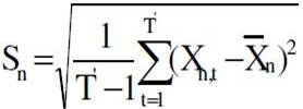
1. For each component n=1,…,15
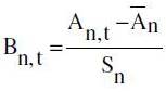 where
where  and
and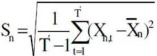
 2. where
 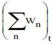 is the sum of the weights of the available series at time t
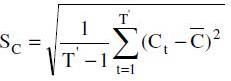
3. 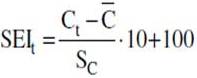 where
where  and
and 
The Xn variables represent the 15 components of the confidence indicators for industry (3 components), services (3), consumers (4), construction (2) and retail trade (3).
Since the confidence indicators described above are made up of the same, but non-standardized component series, the ESI cannot precisely be derived from applying the given sector weights to the five confidence indicators. In fact, it can occasionally happen that, due to the influence of some more volatile component series, the sum of the (weighted) confidence indicators shows movements that are not reflected in the ESI, summarizing the properly standardized components. In the same way, impulses from rather damped components that are not visible in the confidence indicators may actually show up in the ESI.
Simulating the ESI Using ANN
Regardless of the ANN used the processed data or the simulated problem and the phases in the implementation of ANN are the same, as shown by the authors in authors articles.
[Ilie C., Ilie M., Moldova Republic’s Gross Domestic Product Prevision Using Artificial Neural Network Techniques, OVIDIUS University Annals, Economic Sciences Series, Volume X, Issue 1, Year 2010, OVISIUS University Press, p. 667-672, ISSN 1582-9383]. Considering this, the following simulation follows those phases.
Phase 1 — Initial Data Analysis
Data analysis consists in dividing data into separate columns, defining types of these columns, filling out missing number values, defining the number of categories for categorical columns, etc.
Data analysis revealed the following results:
- 6 columns and 79 rows were analyzed;
- Data partition method: random;
- Data partition results: 57 records to Training set (72.15%); 11 records to Validation set (13.92%) and 11 records to Test set (13.92%).
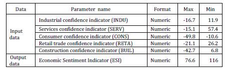
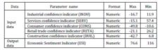
As can be seen, the database is divided in three sets. While the training sets are used only for training, the validation and testing sets are used also for testing. Presented in table 1 are the maximal and minimal value limits of the input and output data.
Table 1: The Database
Phase 2 — Data Pre-Processing
This is the phase in which the above defined data are prepared and reshaped for an easier use and for obtaining best results, according to the requirements and the imposed results.
Pre-processing means the modification of the data before it is fed to a neural network. Pre-processing transforms the data to make it suitable for neural network (for example, scaling and encoding categories into numeric values, “one-of-n” or binary) and improves the data quality (for example, filtering outliers and approximating missing values), as different software uses different methods [see Alyuda NeuroIntelligence – http://www.alyuda.com/neural-networks-software.htm].
“One-of-N” encoding is Method of encoding categorical columns into numeric ones. Each new numeric column will represent one category from the categorical column data. For example, categorical column Capacity that has High, Medium and Low as its values will be encoded into 3 numeric columns and value High will be represented as { 1, 0, 0}, Medium as { 0, 1, 0} and Low as {0, 0, 1}.
Considering the past research and experiences, the database was reorganized as random series replacing the initial time series.
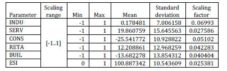
The reasons for this change came from the need to avoid the obstruction of the training and also the probability of the ANN to consider the trend of the time series database as universal trend. The second problem can be determined by the impossibility for future estimates. So the data on which the ANN was trained were fed to it as non-time series; and for the present database, the encoding chosen was numeric encoding. Numeric encoding means that a column with N distinct categories (values) is encoded into one numeric column, with one integer value assigned for each category. For example, for the Capacity column with values “Low”, “Medium” and “High”, “Low” will be represented as {1}, Medium as {2} and High as {3} [Alyuda NeuroIntelligence – http://www.alyuda.com/neural-networks-software.htm]. In table 2, the characteristics of pre-processed data are shown.
The results of completed pre-processing process are:
- Columns before preprocessing: 6;
- Columns after preprocessing: 6;
- Input columns scaling range: [-1..1];
- Output column(s) scaling range: [0..1];
- Numeric columns scaling parameters: INDU: 0.06993; SERV: 0.027586; CONS: 0.05102; RETA: 0.042283; BUIL: 0.040404; ESI: 0.025381.
Table 2: The Pre-Processed Database
Phase 3 — Artificial Neural Network Structure
Considering the characteristics of the simulated process, many ANN structure can be determined and compared through the specificity of the process and the data that are being used for simulations. Thus, the feed forward artificial neural network is considered the best choice for present simulation [Lucica Barbeş, Corneliu Neagu, Lucia Melnic, Constantin Ilie, Mirela Velicu, The Use of Artificial Neural Network (ANN) for Prediction of Some Airborne Pollutants Concentration in Urban Areas, Revista de chimie, Martie 2009, 60, nr. 3, Bucharest, p. 301-307, ISSN 0034-7752].
After building and testing several ANN with feed forward structures, having in mind the comparison of the errors between the real data and ANN output data, the best ANN network was defined. This has the following structure (figure 2): 5 neurons in the input layer, 11 neurons in the hidden layer and 1 neuron in the output layer.
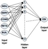
Figure 2. Simplified Graphic Representation of ANN with Structure 5-11-1
Also, the activation function for different layer neurons are chosen: Hidden layers activation function is hyperbolic tangent (ratio between the hyperbolic sine and the cosine functions (or expanded, as the ratio of the half-difference and half-sum of two exponential functions in the points z and —z) and Output layer activation function is logistic (sigmoid curve) [Dumitru Iulian Năstac, Reţele Neuronale Artificiale. Procesarea avansată a datelor (Artificial Neural Network. Advance Data Processing.) Printech Pub., Bucharest, 2000].
Phase 4 — Training
Being an essential phase in the use of ANN, the training must use certain training algorithms which essentially modifies the structural elements of ANN (weights) modified through several iterations. Those modifications establish the future ANN accuracy. For the selected ANN, the most common training algorithm is Back propagation algorithm.
Back propagation algorithm. Back propagation is the best-known training algorithm for multi-layer neura l networks. It defines rules of propagating the network error back from network output to network input units and adjusting network weights along with this back propagation. It requires lower memory resources than most learning algorithms and usually gets an acceptable result, although it can be too slow to reach the error minimum and sometimes does not find the best solution [Alyuda NeuroIntelligence— http://www.alyuda.com/neural-networks-software.htm]. For a quicker training process, a modification of the back propagation algorithm, called quick propagation, was made.
Quick propagation is a heuristic modification of the back propagation algorithm invented by Scott Fahlman. This training algorithm treats the weights as if they were quasi-independent and attempts to use a simple quadratic model to approximate the error surface. In spite of the fact that the algorithm has no theoretical foundation, it is proved to be much faster than standard back propagation for many problems. Sometimes the quick propagation algorithm may be instable and inclined to block in local minima [Alyuda NeuroIntelligence —http://www.alyuda.com/neural-networks-software.htm].
The training conditions were established in order to achieve the best results using the quick propagation training algorithm. Thus, the quick propagation coefficient (used to control magnitude of weights increase) was 0.5 and the learning rate (affects the changing of weights — bigger learning rates cause bigger weight changes during each iteration) was 0.3. The small values of these two, especially of the learning rate, are explained by the necessity of avoiding the local minima blockage.
The results of training details are presented in table 3.
Table 3: The Training Details

- AIC is Akaike Information criterion (AIC) is used to compare different networks with different weights (hidden units). With AIC used as fitness criteria during architecture search, simple models are preferred to complex networks if the increased cost of the additional weights (hidden units) in the complex networks do not decrease the network error. Determine the optimal number of weights in neural network [Alyuda NeuroIntelligence – http://www.alyuda.com/neural-networks-software.htm];
- Iters. are the iterations [Alyuda NeuroIntelligence – http://www.alyuda.com/neural-networks-software.htm];
- R-squared is the statistical ratio that compares model forecasting accuracy with accuracy of the simplest model that just use mean of all target values as the forecast for all records. The closer this ratio to 1 the better the model is. Small positive values near zero indicate poor model. Negative values indicate models that are worse than the simple mean-based model. Do not confuse R-squared with r-squared that is only a squared correlation [Alyuda NeuroIntelligence – http://www.alyuda.com/neural-networks-software.htm];
The stop training conditions were: maximum of 500000 iterations or a maximum absolute training error value of 0.25%. The results of training are Number of iterations: 500001 (Time passed: 00:09:35 min.). The training stop reason was: All iterations done.
Training Results
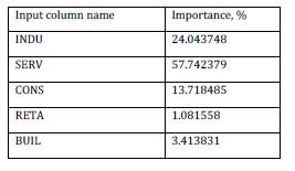
After the training, the ANN evaluated the importance that every input data has over the output data. The result of the evaluation is presented in table 4 and figure 3.
Table 4: Input Data over Output Data Importance
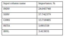
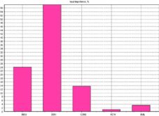
Figure 3. Input Data over Output Data Importance
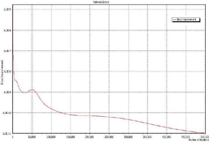
In the next figures, the results of the training are shown as follows: Figure 4: the evolution of network error through the 500000 iteration.
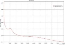
Figure 4. Evolution of the Network Errors
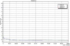
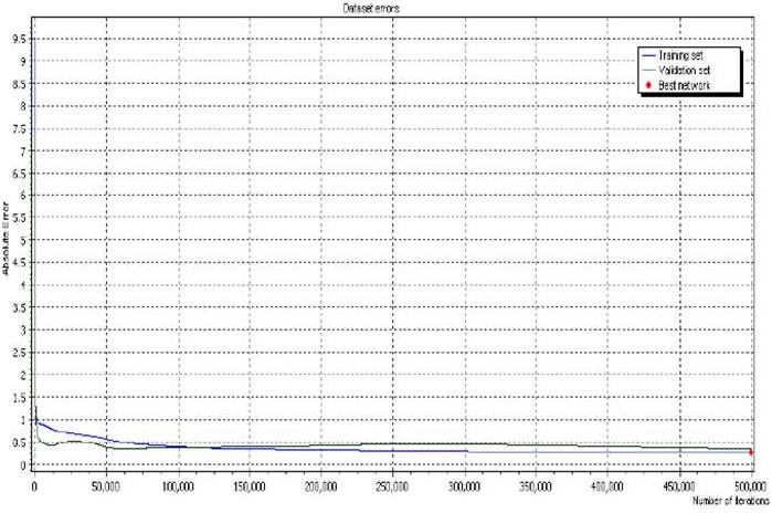
Figure 5. Comparison between Training Set Dataset Errors and Validation Dataset Error

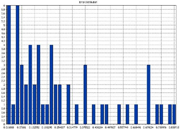
Figure 6. Training Errors Distribution
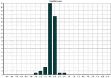
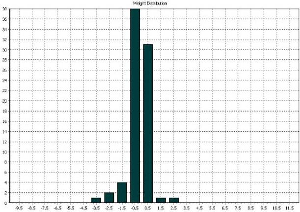
Figure 7. Network Weight Distribution
Phase 5 — Validation and Testing
The last phases of ANN simulation indicate the level of ANN preparedness regarding the expected results.
Testing is a process of estimating quality of the trained neural network. During this process, a part of data that was not used during training is presented to the trained network case by case. Then forecasting error is measured in each case and is used as the estimation of network quality.
For the present research, three different sets of data were used for the testing and validation of the ANN training. The first set is the one already used in the training process, but never fed to the ANN: 11 records to Test set (13.92%) (see phase 1). The results of this testing is presented in table 5. Also the difference between the real values (target) and the simulated values (output) of the output data are presented in figure 8.
Table 5: Test No. 1. Automat Testing Results — Actual Vs. Output
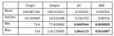
AE is the absolute error as the difference between the actual value of the target column and the corresponding network output, in absolute values [Alyuda NeuroIntelligence – http://www.alyuda.com/neural-networks-software.htm];
– ARE is the absolute relative error as the difference between the actual value of the target column and the corresponding network output, in percentage terms [Alyuda NeuroIntelligence – http://www.alyuda.com/neural-networks-software.htm].
The second set is formed from data that was never fed to the ANN in order to train it. So this set was new to the trained ANN. The results of the comparison between the real data and the simulated data are presented in table 6.
Table 6: Test no. 2. Testing results – Actual vs. Output
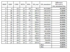
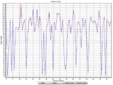
Figure 8. Actual vs. Output Values. Automat Testing
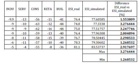
The third set was a new set and when the ANN was trained, this set was not yet revealed on European Commission — Economic and Financial Affairs website [http://ec.europa.eu/economy_finance/db_indicators/surveys/time_series/index_en.htm]. The result of this set on the ESI simulation is presented in table 7. The importance of this test came from the economic Romanian situation at that time, which was slightly different from the ESI point of view. So it was necessary to determine how the trained ANN behave in somehow illogical (the non-linear conditions that we refer to) conditions, such as higher than expected confidence in country’s capabilities.
Table 7: Test no. 3. Testing results – Actual vs. Output
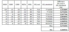
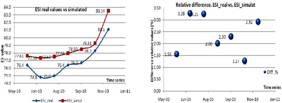
The absolute values and relative difference for the third testing process, between the third real set of values and the simulated ones are shown in figure 9.
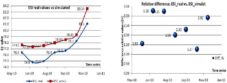
Figure 9. Actual vs. Output Values. Test No. 3
From the previous results, the following conclusions are drawn:
- The training phase was successful, the maximum absolute error was 1.866 and the maximum absolute relative error was 0.016;
- Testing the training with the new data set resulted in a smaller than 3.3% difference between the real data and simulated output.
Simulating the Trend ESI Using the ANN
The researchers did not only evaluate the success of ANN training by comparing the real input data with the ANN simulated data, but they also observed the trend that ANN simulates, considering new data for each of the input.
In order to see the way the ANN behaves after the training, we fed the ANN with the new data, as consecutive values in arithmetic progression, for each and every input, while the other four inputs remained the same as in training session. Then we considered the trend of the new used data in comparison with the real trend. We used the trend of the simulated data because, as expected, the simulated data were affected by the simulation errors and thus the trends will be easier to compare.
The trends were determined using a simple program from the Mathcad 2001 software, for the calculation of the equation that approximates the trend. The results of ESI simulations for the new data were considered (with consecutive values in arithmetic progression and all other inputs remaining as in original database). An example of the program which determined that trend for the INDU input data is presented here in figure 10.
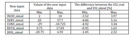
Also, the researchers must explain the interval values chosen for the new simulations. For example, the real values for the INDU data were between [-16.7; 11.9], but we want to verify and test even more the ANN trained with a different values interval. So a new interval for INDU was considered as [2; 10], this interval showed that the trained ANN can simulate using new data that were never fed to it. In addition, the trained ANN simulation can be appreciated considering that all values are only positive and can be found in a smaller cluster than the real data (that were used for training).
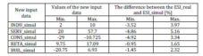
In the following figures the simulated ESI (ESI_simul) is shown for each of the new sets of values for the input data: INDU_simul, SERV_simul, CONS_simul, RETA_simul and BUIL_simul (noted with a) in the following figures) and the trend determined from the simulated ESI (noted with b) in the following figures). Also in order to evaluate the ANN, the difference between the real ESI (ESI_real) and the simulated ESI (ESI_simul) is presented as percentage (noted with a) in the following figures) and also as absolute values graphics (noted with b) in the following figures).
Trend Simulation with New INDU Values
The values for the INDU input data was chosen between [2; 10], the other input data values remained as shown in table 1. The results of the simulation are presented in figure 11.a and the calculated trend in figure 11.b.
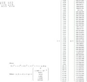
Figure 10. The Program for the Calculus of the INDU’s Trend Equation
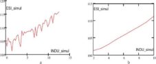
Figure 11. a) ESI Simulated for the New INDU Values; b) Trend of the ESI Simulated for the New INDU Values
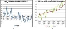
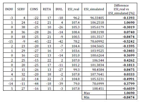
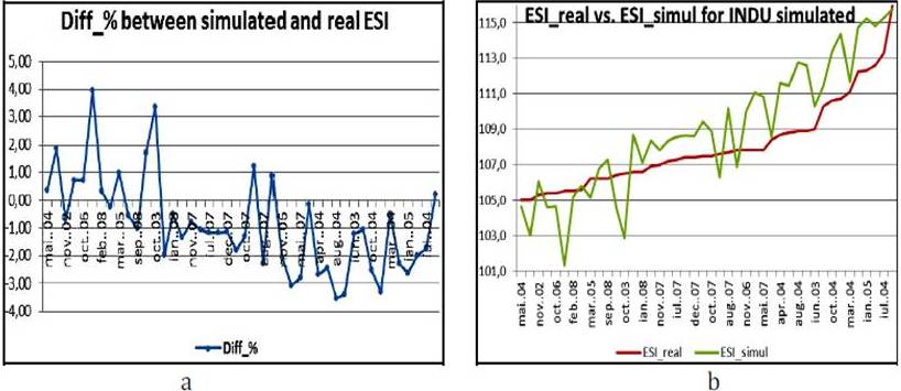
Figure 12. a) The Difference between Simulated ESI and Ral ESI for the New INDU Values (%); b) ESI_real vs. ESI_Simul for the New INDU Values
In figure 12.a, the difference between the real ESI and the simulated ESI as percentage are presented. The difference percentage values were between [-3.52; 3.97]. These values are smaller than the initial conditions regarding the error of the ANN. The absolute values of the ESI_real and the ESI_simul are presented in figure 12.b for a better comparison.
As presented in this section, the figures for the other four input data are presented in the next figures, as follows:
- Figures 13 and 14 for input data SERV;
- Figures 15 and 16 for input data CONS;
- Figures 17 and 18 for input data RETA;
- Figures 19 and 20 for input data BUIL.
For a better view of the new values used for the simulations of the ESI and for the results of that simulations see table 8.
Trend Simulation with New SERV Values
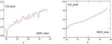
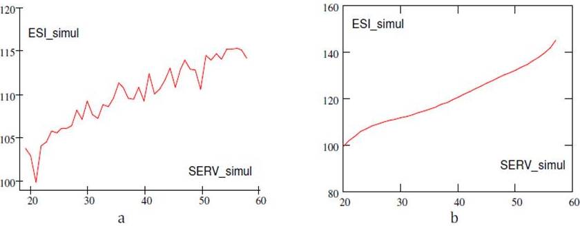
Figure 13. a) ESI Simulated for the New SERV Values; b) Trend of the ESI Simulated for the New SERV Values
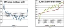
Figure 14. a) The Difference between Simulated ESI and Real ESI for the New SERV Values (%); b) ESI_Real vs. ESI_Simul for the New SERV Values
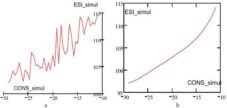
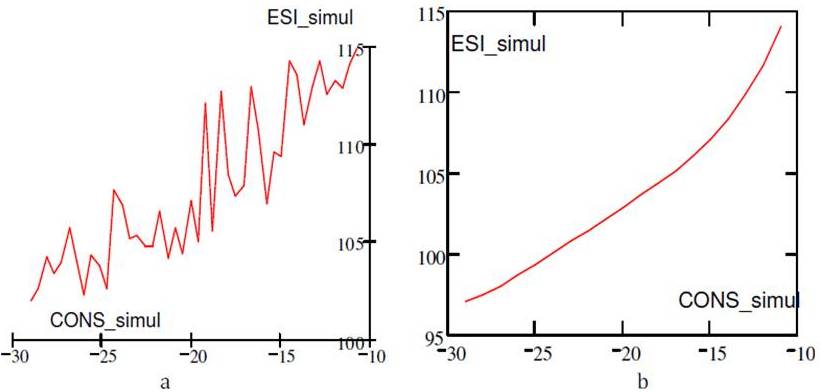
Figure 15. a) ESI Simulated for the New CONS Values; b) Trend of the ESI for the New CONS Values
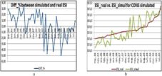
Figure 16. a) The Difference between Simulated ESI and Real ESI for the New CONS Values (%); B) ESI_Real vs. ESI_Simul For The New CONS Values
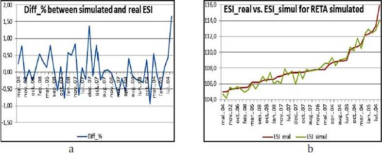
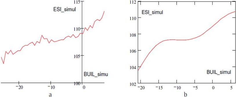
Trend Simulation with New RETA Values
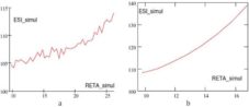
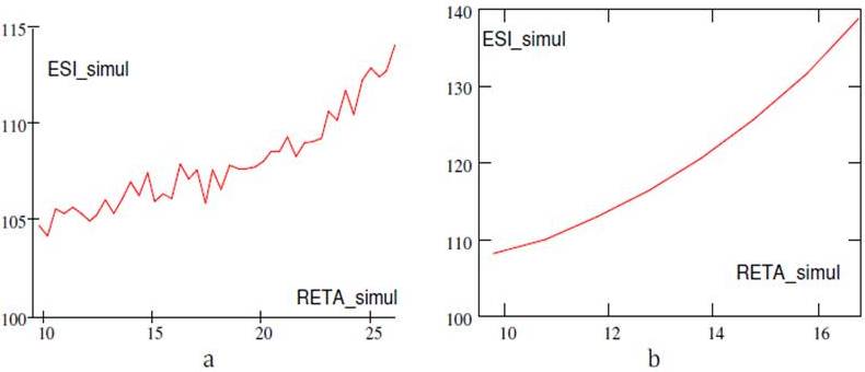
Figure 17. a) ESI Simulated for theNew RETA Values; b) Trend of the ESI Simulated for the New RETA Values.
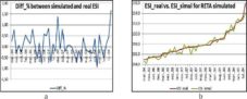
Figure 18. a) The Difference between Simulated ESI and Real ESI for the New RETA Values (%); b) ESI_Real vs. ESI_simul for the New RETA Values
Trend Simulation with New BUIL Values
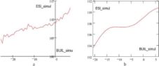
Figure 19. a) ESI Simulated for the New BUIL Values; b) Trend of the ESI Simulated for the New BUIL Values
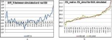
Figure 20. a) The Difference between Simulated ESI and Real ESI for the New BUIL Values (%); B) ESI_Real Vs. ESI_Simul for the New BUIL Values
Table 8: The New Values Of The Input Data Used for The Simulations and The Results of Simulation