Introduction
Modelling of the phenomena following from the economic reality and reflected by the statistical data is based in particular on the mathematic disciplines like statistics, numerical methods, operations research, linear and dynamic programming, optimization, etc. The use of a suitable computer system is inevitable both for modelling, analyses, diagnostics and/or possible solution of issues by quantitative methods, and for economic re-interpretation and application.
The formulation of the new dynamical model of the “shipbuilding cycle” requires the use of analytic and synthetic methods, dynamical modeling and solving the delay differential equations. For numerical solution of the envisioned task for the delay differential equation is used the approach derived from current studies regarding solution of boundary value tasks for systems of „functional differential equations“.
The use of a suitable computer system is inevitable both for modeling, analyses, diagnostics and/or possible solution of issues by quantitative methods, and for economic re-interpretation and application. The aim of submitting the article is to present possibilities of current software, to describe their use for applications and show how to construct a realistic model, which takes into consideration the data from previous periods expressed by a delay differential equation.
Finding the mathematical programs include in general also the graph creating programs (e.g. Graph, Gnuplot), statistical programs (e.g. Statistica, Origin, SPSS) and/or the programs specialized on numerical computations (e.g. Matlab, Scilab, Maple). The Maple system grants effective tools for solution of differential equations of more types. For solving of delay differential equations there is only one procedure for solving of delay differential equations in Maple, namely “method of steps”. For this we can successfully use standard functions.
The paper presents possibilities of software solutions of dynamical economic models by means of delay differential equations (DDE). The aim of the paper is to present possibilities of the Maple system in solving differential equations with delay and consequently the possibility of graphical presentation of results. In our paper it will be discussed in detail the possibility of using Maple system for solving the model of Tinbergen’s “Shipbuilding cycle”.
Modeling in Economy
Many economists have their own specific definitions of economic models. The following definitions are taken from several economic publications:
Samuelson and Nordhaus (2009) gave the definition of a model as a formal framework for representing the basic features of a complex system by a few central relationships. Models take the form of graphs, mathematical equation, and computer programs.
Begg, Fischer, and Dornbusch (2000) found that a model or theory makes a series of simplification from which it deduces how people will behave. It is a deliberate simplification of reality.
Economists and mathematicians have long been trying to use dynamic systems in economics. Dynamic processes in economy and the existence of economic cycles were identified by French physicist C. Juglar in the first half of 19th century. His ideas were then elaborated on (van Gelder, 1913) and (Kitchin, 1923). This in whole opened a new path for the theory of economy dynamics represented for example by S. Kuznets (1930, 1940), J. Mensh (1975), A. Klainkneht (1981) or J. van Duijn (1983). The second half of twenty century brought about the development of not only electrical engineering, mechanics and chemical engineering, but also biology, ecology, medicine, mathematical economics (Doubravsky, Doskočil, 2011) and many other fields of science and technology (for respective examples and references see (Andejev 1992), (Titov 1996). The dynamic economics was brought to the attention of J. Schumpeter (1987), who refined economic analysis, converting to dynamics, connecting economics, history and sociology.
Modern representative of the long-wave theory, Ch. Freeman points out the influence of employability and analyses effects of innovation waves on its’ increasing, resp. declining in the spirit of Keynesian full employment drive (Freeman, 1996). Forrester’s and Freeman’s theories, in accordance to multiplier-accelerator theory were worked out by J. P. Samuelson and Hicks (Samuelson, 1939). Samuelson-Hicks model and also Phillips model of accelerator-multiplier are dynamic revenue models, based on Keynesian school, used for determination of revenue prediction in dependence on starting conditions and structural constants of given economy.
Major contribution to the accelerator-multiplier was made by Nikolas Kaldor, a famous British economist, who used to criticize the original model for its excessive simplicity. According to Kaldor (1940), the theory should have been based on non-linear investment function. Polish economist Michael Kalecki worked on the theory of business cycles for Poland (Kalecki, 1935). In his works, he distinguished several versions of the dynamic model: linear, non-linear and linear with exogenous shock.
In their monograph, Kobrinskij and Kuzmin (1981) pointed out the necessity of using variables of historic type in dynamic economic models that have impact on system development and leads to major changes in the character of the entire process. In Simonovs studies, (Simonov, 2002a, 2002b, 2003) has modified existing micro and macro economical models, such as Walras-Evans-Samuelson (WEC) model with regard to delay between offer and demand, Allen’s model on the single-commodity market, with regard to delay of deliveries and dependence of demand and offer on the price and speed of price changes (Alen, 1963), Vidal-Wolf’s model of single-product sale Dychta and Camsonjuk (2003) etc.Some authors are currently returning to Kalcecký’s model using delay differential equations (i.e. Asea and Zak (1999), Collard et al. (2008)).
Shipbuilding Cycle from the View of Jan Tinbergen
In this paper, we want to deal with one of Tinbergen’s big issues, the shipbuilding cycle. In the article named “A Shipbuilding cycle?” (1930) the author demonstrates a relationship between shipbuilding and freight rates as a type of “elementary fluctuation”. Jan Tinbergen is concerned with this topic because it displays interesting characteristics of consequence to the theory of economic fluctuations in general, and also has a significant meaning for the field of shipbuilding.
According to Tinbergen, fluctuations in shipbuilding determine to a great extent the fluctuations in the increase in total tonnage of a country’s merchant marine. The volume of shipbuilding is largely dependent on the level of freight rates. These in turn are correlated with total available tonnage. An increase in tonnage would probably appear about one year after the occurrence of increased rates, because one year was in the thirties of the last century the construction time of a new ship. This phenomenon can be termed as lag correlation.
The relationships described above are the basis for the most significant one — the relationship between the increase in total tonnage and the volume of the total tonnage of about two years earlier.
It also has the social and economic significance which Tinbergen describes as follows: the volume of shipbuilding is primarily a function of the ship owner’s demand for freight capacity, and furthermore, the level of freight rates depends mainly on the ship owner’s supply of freight capacity. The demand of importers and exporters considered as an aggregate fluctuate much less. The effect of other factors is secondary.
The previously mentioned relations result in the following scientific problem: how great would the total tonnage and its rate of increase have been if the described relations had had no exceptions? This relationship, Tinbergen calls it the “reaction mechanism”, will in most cases prove to result in a cyclical movement which is named as “the shipbuilding cycle”.
Tinbergen’s Way of Solving Equations of the “Shipbuilding Cycle”
Tinbergen wants to obtain the development over time of total tonnage; time will be expressed as t, tonnage as y(t), so that the function f is our unknown quantity
The Tinbergen’s equation (Tinbergen, 1931) is of the form
y´(t) = −ay(t −ï„), b > 0, (1)
The solution of equations of this kind (functional equations) in analytical mathematics was not found “methodically” but experimentally in Tinbergen’s article.
It is also assumed that
y(t) = h(t), t  <0,Δ), (2)
Where h(t) is some given function. In this application to the shipbuilding industry, y denotes the deviation of the tonnage from a mean value and a given constant construction time. In this equation, Tinbergen assumes the rate of new shipbuilding to be proportional to a delayed tonnage deviation, with a one to two years delay and a ranged intensity reaction b.
Tinbergen shall try to give an explanation of the most important features of equation for economic theory and, in particular, the theory of trade cycles in nonmathematical terms. The fluctuations following the law of the “shipbuilding mechanism” are determined by:
– the delay Δ,
– the intensity of reaction a,
– the movement during an “initial period” from which point on wan the mechanism has been undisturbed.
The “initial development” determines the relative importance of the components. The importance of the bigger cycles will be greater if the smaller ones in the initial development are not recognizable. In the present case of shipbuilding the periods which are shorter than two years (Δ < 2) in connection with the “mechanism” are probably insignificant.
Tinbergen describes four cases of parameter aΔ values:
1. aï„ â‰¤ 1/e ≈ 0.37, in other words in the case of short lags and/or small intensity of reaction there is no cyclical motion, just a unilateral adaptation to the state of equilibrium y(t) = 0, i. e. to the trend.
2. aï„ ïƒŽ (0.37, Ï€/2), then we get a damped sine wave, i. e. a gradual approximation to the state of equilibrium by the steadily decreasing amplitude of the fluctuations.
3. aï„ = Ï€/2, we get a pure sine wave, that is to say, a cyclic motion with constant amplitude.
4. aï„ > Ï€/2, we get sine waves with amplitudes increasing in time.
5. In the latter two cases therefore there is no approximation to a state of equilibrium.
Results at which Jan Tibergen arrived experimentally are consistent with the results of properly derived mathematical statements (e.g. M Marušiak, 2000).
Suitable Software for Mathematical Modeling
There is a great amount of mathematical programs capable of solving different concrete tasks, because they have historically been developed by different universities and are thus orientated on solving of different problems. In general, mathematic programs include programs for graph generating (i.e. Graph, Gnuplot), statistic programs (i.e. Statistica, Origin, SPSS), alternatively programs specialized on numerical calculations (i.e. Matlab, Scilab, Maple). More complex mathematical programs allows not only to solve equations and work with algebraic expressions, but also can do integral and differential calculus, graph drawing, work with units, interactive document change, numerical calculations and much more.
It is necessary that the selected provide comfort during solving differential equations for the purpose of our article. We can choose Maple from the available software.
Maple is the leading multipurpose mathematical software tool. It provides advanced high performance mathematical engine with fully integrated numeric and symbolic, all accessible from WYSIWYG document environment. But this software doesn’t contain a procedure for dealing with this type of equations, which is a big disadvantage of this tool.
Differential Equation in Maple
The Maple system grants effective tools for solution of differential equations of more types. Prior to start work with the differential equations, it is always necessary to activate the DEtools package in the notebook, using the command with (DEtools). This package contains the commands which we will work with, when solving the differential equations.
The commands diff, Diff and D are usually applied for the derivation itself. In this paper the command diff will be used for further calculations. The expression is considered its argument; it is written in the form diff (expression, variable).
If we want to determine the kind of the differential equation, we use the command odeadvisor classifying the said equation.
Dsolve, having a number of optional arguments, is the basic command for solution of differential equations. When solving the system of differential equations, the dsolve command can include the lists of more parameters of the same type in the brace(s). The form looks then as follows:
Dsolve ({list of differential equations, list of initial conditions}, {unknown functions}, other arguments).
Solution of the said equation can also be presented, using the commands deplot, odeplot or phase portrait. The command plot, used in general for plotting graph of the function in the Maple programme, cannot be applied here directly.
The command odeplot – from the plots package – is used for plotting one or more graphs of the numerical solution with the initial conditions. Output of the command dsolve is the mandatory parameter for this command, axes and functions of the variables to be plotted, scope of axes where the graph is plotted and other graph parameters which are the same like for the command plot are considered the optional parameters.
For the deplot (also DEplot) command, unlike the odeplot command, differential equations or the system of differential equations and the initial conditions are the mandatory argument. There are many optional arguments for the deplot command, modifying the graph environment.
Analysis of the Equation Solution Using the Modern Theory and Maple
For differential equations with delay exist in Maple procedure for the “method of steps”. It is defined that can be used to compute solutions of the scalar linear delay differential equation with constant delay.
The method of steps is an elementary method that can be used to solve some DDEs analytically. DDEs that arise most frequently in the modelling literature have constant delays. This method is usually discarded as being too tedious, but in some cases the tedium can be removed by using computer algebra.
A comprehensive and complex analysis of dynamic argument equations was made by attendants of the Permu seminar (Azbelev, 2001), (Azbelev 2003), the results were then systematised in monographs (Azbelev, 1991), (Azbelev, 2002).
At times when analytical solutions for functional differential equations are hard and almost impossible to find, scientists and engineers resort to numerical solutions that can be made as accurately as possible.
The numerical solution to the given problem of a system of differential equations with delay argument used a method derived in current studies on solving boundary value problems for systems of so-called functional differential equations — see (Kuchyňková and Maňásek, 2006).
Monograph Kiguradze and Půža (2003) contain general theory which allows solving not only the problem above but also others. The application of the above types of delayed differential equation including the description of method of construction the desired solution, as Kuchyňková and Maňásek (2006) and literature cited there.
In our article we will analyse the problem mentioned earlier using the modern theory of functional differential equations, of which a very special part is the theory of linear differential equation with delay.
We will use the fact that the conventional, numerical solutions are adapted for DDEs from the existing numerical solutions for ordinary differential equations.
For solution of common differential equations and their system, Maple uses the dsolve function. It can search for solution both numerically and statistically, concrete solution path is based on the definition (and specification) of additional function arguments. With each single numeric method we can specify various parameters that will affect the solving run. Specifically we can set speed, accuracy, but also the final shape of method.
Illustrative Example:
Given existing possibilities provided by functional analysis and the theory of differential equations with delay, it is possible to obtain a wider spectrum of results and compare the influence of various parameters. This paper focuses on the fact that in his article Tinbergen describes a solution of equation (1) not allowing for “historic development” in time t < 0. Assuming that changes in values known from the past can be described by a suitable function; we can take advantage of modern theory and solve the whole problem taking the development into account.
In order to demonstrate possibilities of the new approach to the solution of the original problem, let’s assume that the “historic development” prior to time t = 0 can be simulated by function y = sin(t). In order to make the comparison of particular results simpler for different values of parameter a, an identical time delay and display in one graph were used. Parameter aï„ was selected according to Tinbergen’s findings aï„ < 1/e, 1/e < aï„ < Ï€/2, aï„ = Ï€/2 and aï„>Ï€/2.
We also choose the parameter ï„ = 2 (the value Tinbergen came out from).
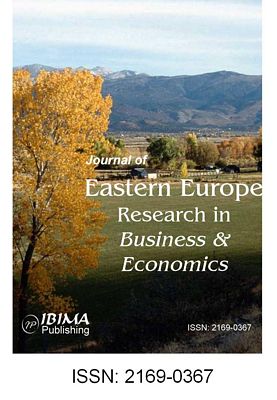
Figure 1 : Solving differential equations using Maple (Source: author’s own study)
Solution in Maple
In Maple exists an opportunity to use a function for solving differential equations with delay, which solves this type of equation by the step method. The above mentioned theory will be transferred to the solution of differential equations with delay due to the limitations of this method. Then, we can apply common numerical methods of solving the ordinary differential equations in Maple (see Fig 1).
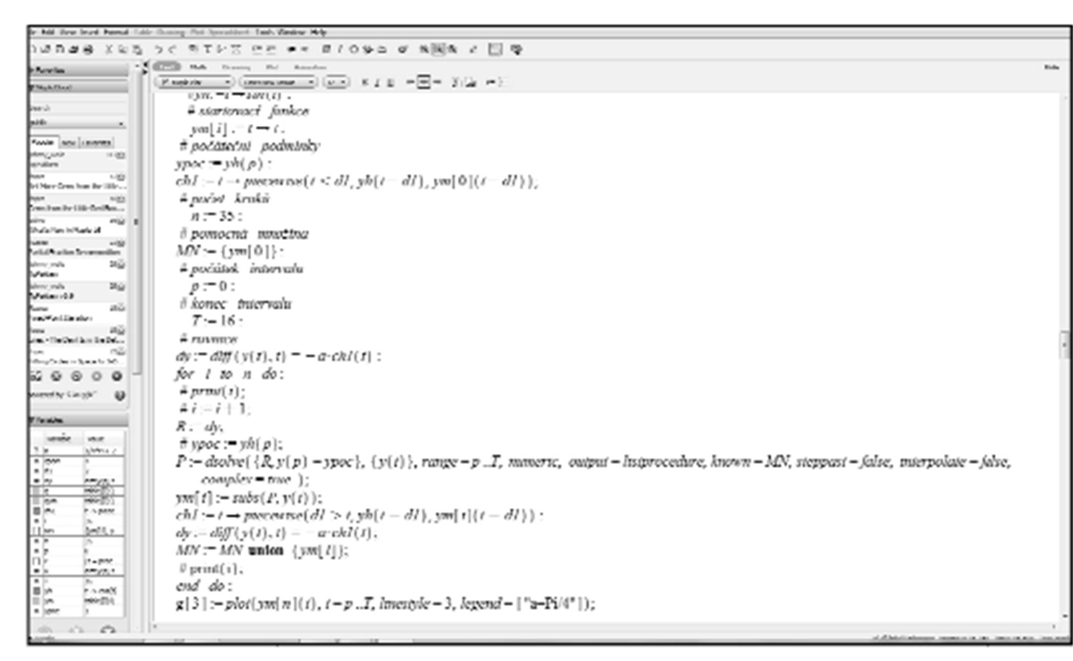
Figure 2 : Approximation 1-35. (Source: author’s own study)
Capabilities of package plots were used for graphical solution, it allowed to make a conclusion about the impact of changes in parameter a on a solution
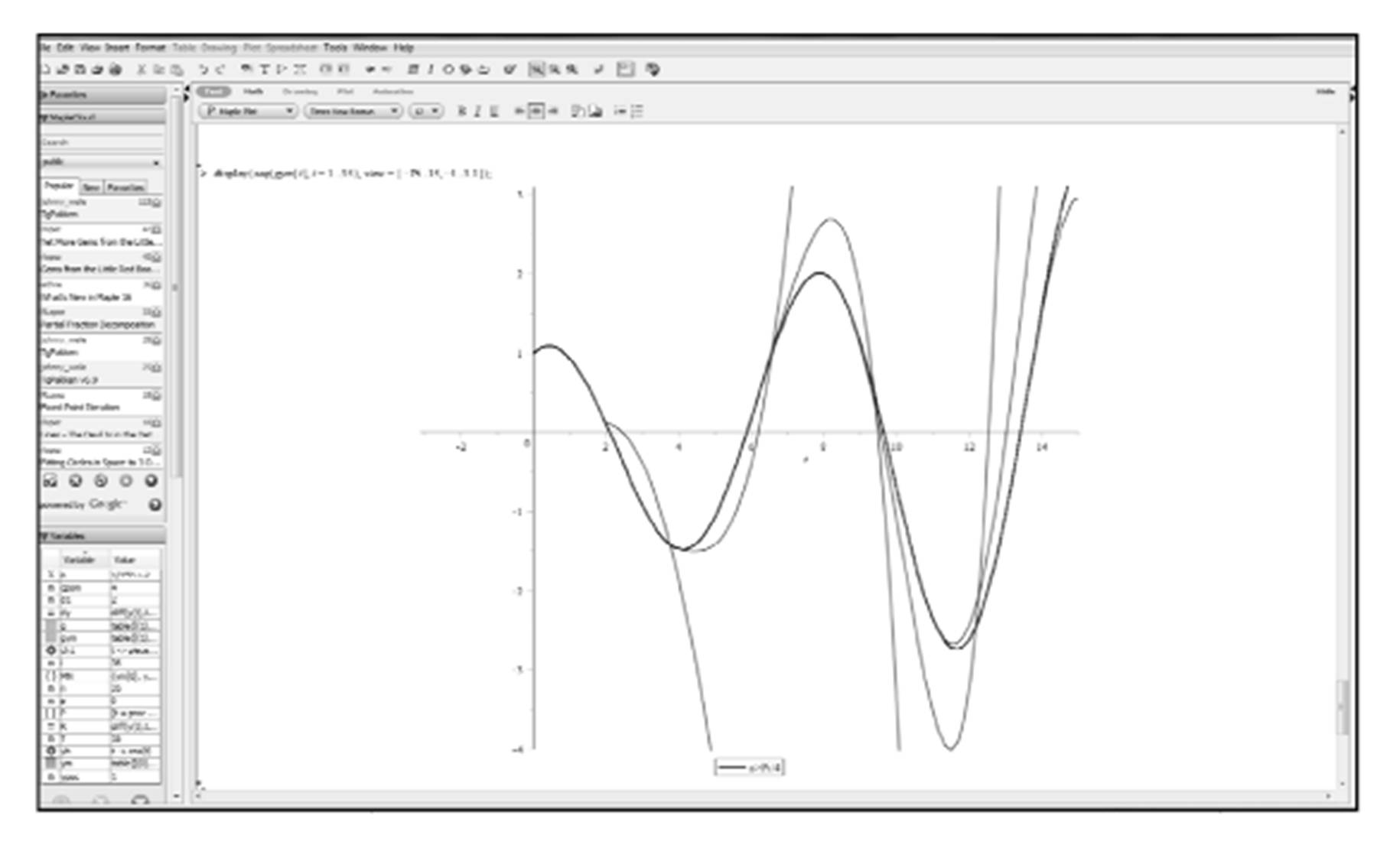
Figure 3: Behaviour of chart in case of change of a parameter a. (Source: author’s own study)
As the graphs show, the value of parameter a significantly influences the length of the “shipbuilding cycle” and it holds true that the higher the value of aï„ is the shorter the cycle gets. The graphs Fig 3 were plotted on the assumption that ï„ = 2 (which is a value that Tinbergen also proceeded from). The cycle, apparent on the graphs, is clearly in accordance with Tinbergen’s findings. This fact is supported by comparison of Tinbergen’s original outline and Maple output.
Conclusion
When modelling complex economic problems we have to face the fact that relations between particular quantities change in time. Such dynamic character can be captured by allowing for a “delayed effect” of exogenous and endogenous variables when specifying the structure of a model. Also, time is regarded as continuous quantity and such dynamic models are described using differential equations.
This paper pointed out the possibilities of the application of the modern theory of differential equations with delay in economic modelling. It has also been demonstrated on original Tinbergen’s problem that the original solution can be successfully extended, and significantly more precise information can be thus obtained on the behaviour of the model concerned. Specific results are given for the illustrative example and thanks to computer processing of the problem the results can be presented in graphic form.
When creating the models, the theoretic solution of the set task itself is not the sole problem; choice of the tool serving for calculation of the parameters necessary for adequate description of the model must be considered as well. Aim of the article was to familiarize the reader with the procedure of solving economic model using differential equation in Maple. The solution was described using graphical representation of the result. The paper was unable to describe in details all the commands and their parameters that had to be applied for the solution. Despite this restriction the reader should be granted the adequate information necessary for independent solution of similar issues
It can be stated in conclusion that the Maple system is very user friendly even for the beginners and enables to obtain the underlying documents for further decision taking in a relatively comfortable way. It becomes a suitable variant supporting utilization of the exact methods of modelling in the economic practice. The user shall only perform interpretation of the obtained results.
Acknowledgement
This paper was supported by grant FP-S-13-2148 ‘The Application of ICT and Mathematical Methods in Business Management’ of the Internal Grant Agency at Brno University of Technology.
References
1. Allen, R. D. G. (1971) ‘Matematická ekonomie’. Praha: Academia.
2. Andreeva, E. A., Kolmanovskij, V. B. and Sajchet, L. E. (1992) ‘Upravlenie sistemami c posledejstvem’, Ðœoskva: Nauka.
Publisher – Google Scholar
3. Asea, P. K. and Zak, J. P. (1999) ‘Time-to-build and cycles’, Journal of Economic Dynamics and Control, 23(8), 1155-1175.
Publisher – Google Scholar
4. Azbelev, N. V. (2001) ‘K 25-letnju Permskogo ceminara po funkcionalno-differencialnym upravnenijam’, Differenc. Upravnenija, 37(8).
5. Azbelev, N.V. (2003) Kak eto bylo (ob osnovnych etapach pazvitija sovremnnoj teorii funkcionalno-differencialnych upravnenij), Problemy nelinejnnogo analyza v inženernych sistemach, 9(17).
6. Azbelev, N. V., Maximov, V. T. and Rachmatullina, L.F. (1991) ‘Vvedenie v teoriuju funkcionalno-differencialnych upravnenij’, Ðœoskva: Nauka.
7. Azbelev, N. V., Maximov, V. T. and Rachmatullina, L. F. (2002) ‘Elementy sovremnnoj teorii funkcionalno-differencialnych upravnenij: Metody I prilozenija’, In-t kompjuter. 2002.
8. Begg, D., Fisher, S. and Dornbush, R. (2000) Economics, 6th ed. McGraw-Hill.
9. Collard, F., Licandro O. and Puch L. (2008) ‘The short run dynamics of optimal growth models with delays’, Annales d’Economie et Statistique, 90, 127-144.
Google Scholar
10. Doubravský, K.; Doskočil, R. (2011) Accident insurance – a comparison of premium and value of the vehicle. Innoviation and Knowledge Management: A Global Competitive Advantage. Kuala Lumpur, Malaysia, International Business Information Management Association. p. 1248 – 1258.
11. Duijn, J. J. (1983) ‘The long wave in economic life’, George Allen &Unwind.
12. Dychta, B. A. and Camsonjuk, O. N. (2003) ‘Optimalnoe impulsnoe upravlenie c priloženijami’, Moskva: Fizmatlit.
13. Freeman, C. (1996) ‘Long wave theory’, Cheltenham, UK: Edward Elgar.
14. Van Gelderen, J. (1913) ‘Springtide: reflections on industrial development and price movements’ De Nieuwe Tijd 18, 55(3).
15. Juglar, C. (1862) ‘Des Crises commerciales et leur retour periodique en France’, en An-gleterre, et aux Etats-Unis.
16. Kaldor, N. (1940) ‘A model of the trade cycle’, Economic Journal, 50, 78-92.
17. Kalecki, M. (1935) ‘A macrodynamic theory of business cycle’, Econometrica, 3, 327-344.
18. Kiguradze, I. and Půža, B. (2003) ‘Boundary value problems for systems of linear functional differential equations’, Folia Fac. Sci. Mat. Masarykianae Brunensis, Mathematica, 12.
Google Scholar
19. Kitchin, J. and Mills, T. C. (1923) ‘Cycles and Trends in Economic Factors’, The Review of Economics and Statistics, 5(1), 10-16.
20. Kleinknecht, A. (1981) ‘Observations on the Schumpeterian swarming of innovations’, Kobrinskij, N. and Kuzmin, V. (1981) ‘Točnost ekonomiko-matematičeskich modelej’, Moskva: ProgressFutures, 13(4), 293-307.
21. Kuznets, S. (1930) ‘Equilibrium economics and business-cycle theory’ The Quarterly Journal of Economics, 44(3), 381-415.
Publisher – Google Scholar
22. Kuznets, S. (1940) ‘Schumpeter’s business cycles’, The American Economic Review, 30(2), 257-271.
23. Marušiak P. and Olach R. (2000) ‘Funkcionálne diferenciálne rovnice’, EDIS, Žilina,
24. Mensch, G. (1975) ‘Das technologische Patt: Innovationen überwinden die Depression’, Frankfurt-am-Main: Umschau Ferlag.
25. Samuelson, P. A. (1939) ‘Interaction between the multiplier analysis and the principle of acceleration’, Review of Economics and Statistics, 21 (2), 75-78.
26. Samuelson, P. A. and Nordhaus, W. D. (2009) Economics, 19th ed, Irwin/McGraw-Hill.
27. Schumpeter, J. A. (1987) ‘Teória hospodárskeho vývoja’ (from german orig: Theorie der wirtschaftlichen Entwicklung), Bratislava: Pravda.
28. Shampine, L. F. and Thompson, S. (2001) ‘Solving ddes in Matlab’, Applied Numerical Mathematics, 37(4), 441-458
29. Simonov, P. M. (2002) ‘O nekotorykh dinamicheskich modeljach mikroekonomiki’, Vestnik PGTU 2003.
30. Simonov, P. M. (2002) ‘O nekotorykh dinamicheskich modeljach makroekonomiki’, Perm: Un. T. Perm.
31. Simonov, P. M. (2003) ‘Issledovanie ustoichivosti rešenij někotorych dinamičeskich modelyach mikro – i makroekonomiki’. Vestnik PGTU 2003.
32. Tinbergen, J. (1931). ‘A Shipbuilding Cycle?’ In Klaasen, L. H., L. M. Koyck and Witteween H. J. (eds.) (1959) Jan Tinbergen – selected papers, North-Holland Publishing Company, Amsterdam.
33. Titov, N. I. and Uspenskij, V. K. (1969) ‘Modelirovanie system s zapazdyvaniem’, Moskva: Energia.