Introduction
The business cycle issue has been a part of the economists’ core-preoccupations since the very first beginning. A phenomenon of such complexity which influences the economic process in all its aspects cannot be the result of a single cause. Sinusoidal movements of production output, interest rates, inflation and unemployment are describing the business cycle found in all market-economies; in other words, it is known that these movements have a cyclical characteristic which outlines the alternation between expansion and depression phases with some regularity. Thus we may assume that through its complexity, business cycle is a bottom pillar of every market economical process.
From this perspective the economists that studied the phenomenon give various explanations and offer different paths to manage with the effects that cycle phases has on the economy, many of these ideas being divergent based on the logic and ideology in which they believe.
In extension of the theoretical constructions on business cycles, the analysis of the phenomenon is completed by empirical tests designed to classify, quantify and explain the various stages of the cycle. Their role lies in an attempt to foreword the emergence of depression moments in an effort to “sweeten” the disruptive effects that economic crisis may have on whether capital or goods and service market. Therefore, the recent literature developed a number of models used for studying the regularity with which the various stages of the cycle are succeeded. Such studies are made by CEPR in Europe and NEBR in USA, which regularly review economic cycles in their chosen areas using data from OECD, Eurostat or other such institutions. For example, CEPR, in the same line with NEBR, defines recession “as a significant decline in the level of economic activity, spread across the economy of the euro area, usually visible in two or more consecutive quarters of negative growth in GDP, employment and other measures of aggregate economic activity for the euro area as a whole, and reflecting similar developments in most countries” (CEPR, 2003). The moments of expansion and contraction are expressed by ascending or descending intervals delimited by points of peak and through.
Using three indicators like growth in GDP, industrial production and employment, in this paper we will analyze the business cycle of two EU economies (France and Romania). Thus, the article will be structured as follows: in the next section we will review the literature in the field; third section will describe the methodology used in our study, followed by the final section, the paper’s conclusion where we will highlight some recommendations.
Literature Review
Beginning with the work published by Burns and Mitchell in 1946, many specialists fixed an aim hardly attainable: to explain the way in which present and future events may affect the real economical flows. For this study we will make use of Burns and Mitchell’s definition (1996) according to which: “Business cycles are a type of fluctuation found in the aggregate economic activity of nations that organize their work mainly in business enterprises: a cycle consists of expansions occurring at about the same time in many economic activities, followed by similarly general recessions, contractions, and revivals which merge into the expansion phase of the next cycle; this sequence of changes is recurrent but not periodic; in duration business cycles vary from more than one year to ten or twelve years; they are not divisible into shorter cycles of similar character with amplitudes approximating their own”.
In this way, the characteristics of the two authors mentioned above are actually the starting point for further analysis. Showing the same passion and guidance the study made by National Economic Bureau of Research (NBER) gives us a chronology of business cycles, a real effort toward establishing minimum and maximum points of it from 1854 until the summer of 2009.
In another publication Jean-Philippe Cotis and Jonathan Coppel (2005) define business cycles “as a regular and oscillatory movement in economic output within a specified range of periodicities”. The Business Cycle Dating Committee defines recession as a “significant decline in the level of economic activity spread across the economy of the euro area, usually visible in two or more consecutive quarters of negative growth in GDP, employment and other measures of aggregate economic activity for the two areas as a whole and reflecting similar developments in most countries”.
As we can see there have been different approaches for analyzing business cycle phenomena. Once entered in the analysis perimeter we find an alternative approach of the business cycle due to Sargent and Sims (1977). Their analysis consists in formulated an dynamic factor model which describe the cyclical behaviour of a key set of time series in terms of a low-dimensional vector of unobservable factors and a set of idiosyncratic shocks.
More recent studies like one’s made by Benczur and Ratfai (2009) examine the business cycle characteristics using 62 countries in their dataset. The study aimed at revealing the sources of cyclical fluctuation in industrialized and emerging market economies.
Other studies have focus on examine the stylized facts of business cycles. For example studies made by Artis and Zhang (1997) or Artis et all. (1997) provide an analysis not only of the volatility but also on the persistence of the business cycles. There is a large literature that has focus on analysing the business cycles synchronization. Berger de Haan and Inklaar (2002), Savva, Neanidis and Osborn (2007) used the industrial production index to characterize the business cycle phenomena.
Methods of Detrending the Business Cycles
In order to extract the time series two unobservable components, trend and cyclical component, we desire to examine in this paper some of the most popular approaches that have been proposed in the literature.
In order to determine the economic cycle, authors like de Haan Berger and Inklaar (2002), Furceri and Karras (2006), Christos S. Savva, Kyriakos C. Neanidis, Denise R. Osborn (2007) Van Aarle et.all. (2008), Alfonso and Furceri (2009) have used various methods of analysis aimed at extracting long-term component of a data series.
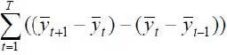
In the literature analysts usually appeal to four different methods in order “to detrend the output series and obtain a measure of the cyclical fluctuation of each series” ( Furceri, Karras, 2005, 2006). The first one refers to a first order difference, using as main indicator the growth rate of real annually GDP. In order to calculate the first order difference (D1) and the year-on-year difference we do not have to relay our analysis on a sophisticated statistical framework for extracting trend and cyclical component but mostly on an intuitive interpretation. (See Furceri and Karras (2006), Van Aarle et.all (2008), Alfonso and Furceri (2009), etc.) The second consists in decomposition of the series into two components: a trend and a cyclic component using the Hodrick Prescott filter method of analysis. Once entered in this analysis perimeter authors like Christos S. Savva, Kyriakos C. Neanidis, Denise R. Osborn (2007), etc. presents an analysis of synchronization of business cycles between the euro area including also recently acceded countries. The time period analysis is wide enough to leave sufficient observations being from 1980-2006. The authors above used in their analysis as the main indicator, industrial production index, applying an HP filter and also the bivariate VAR-GARCH model in order to capture the variation of the correlation coefficient. Berger de Haan and Inklaar (2000, 2002) were used in their analysis as a measure of aggregate economic fluctuations, the index of industrial production for a period from 1990 -2001. Their methodology involves the use of a cyclic index which takes the form set out in Artis and Zhang (1997, 1999) as follows:
Where, Xt- represents the raw series and TREND t the detrended series.
For the analysis the authors mentioned above have used the data provided by International Monetary Fund. Their main results show that “whereas some countries have a more similar business cycle with Germany after the establishment of the ERM, other show a decline in business cycle synchronization.” Also, their analysis shows that in the ERM “….exchanges rates were not uniformly stable just as rates in the pre-ERM period were not fully flexible” (Berger de Haan and Inklaar, 2000, p.16). This perspective shows that the exchange rate stability is not related to business cycles synchronizations.
A third method refers to the filter proposed by Baxter and King (1995) meaning Band Pass Filter (BP). The aim of both authors is to develop and implement a filter that can isolate business cycle fluctuations, “by simply applying moving averages to macroeconomic data” (Baxter, King, 1995, p.3).
On the philosophy branch of the business cycles set by Burns and Mitchell (1946), the above authors presents an alternative method which needs to fulfil six objectives: a) first concerns the removal of a specified range of periodicities; b) the second objective concerns that the ideally band-pass filter should not introduce phase shift; c) the third requires that the method used should be an optimal approximation of the ideal band-pass filter; d) approximation of the filter should result in a stationary time series meaning that this filter implies the eliminations of the quadratic trend from the series; e) the method should yield business cycle component that are unrelated to the length of the sample period; f) the method should be operational (Baxter, King, 1995, pp.3-4).
The method that Baxter and King developed involves applying a moving average to the original time seriesYt, which produce a new time seriesYt*:
 due to the fact that
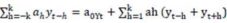
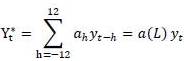
If we take L as the lag operator and applied the filter to the quarterly date, the filter will have the form of the 24- quarter moving average meaning that:
Having L as the lag operator and a(L) =  , after simplications the filter can be factorized as: a(L)= – (1-L)(1-L-1) Æ›K(L) where:
ƛK(L)- simetric moving average, K-1 lags and leads.
The weights of ah can be derived from the inverse Fourier transform of the frequency response function (see also Priestley, 1981, p.274).
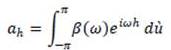
For an ideal filter we have to take into account: a0=ÏŽ/Ï€ și ah=sinâ¡ (hω) / hÏ€; (where h=1,2,…..)
The forth method imply the use of Henderson filter (1916), method used in the seasonal adjustment packages such as X-11 ARIMA, X-11-ARIMA88 and X-12-ARIMA or those that rely on the decomposition of the series, for example by using the program STAMP (see Findley et.al.1998);
Methodology
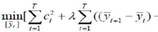
To Lucas (1997) “business cycles are driven by aggregate shocks, not by sector-specific shocks”. Thus, the aggregate cycles are nothing more than real production deviations from the trend. The trend can be identified by applying the Hodrick-Prescott filter (HP). This consists in a time series decomposition of two unobserved components: stochastic trend and a cyclical component, which can be synthetically expressed in the following form:
Yt = µt + Ct
In which: µt — represents the stochastic trend, and Ct the cyclical component
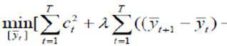
The trend (µt), is potential GDP determined in a way that minimizes the bellow sum. The mathematical representation of this filter is obtained through the minimization of a function with this form:
In which:
T- The total deviation number;
λ – Controls the smoothness of the adjusted trend series

– Represents the sum of squared deviations
-Represents the sum of the long-term changes of trend growth rate.
To determine the business cycle in this analysis we will make use of HP filter in which for parameter that penalizes fluctuations in the growth component time series we will use the recommended HP values: λ = 1600, for quarterly series and for monthly series the value used will be 14400. The value of this parameter may be obtained using the following:

The more value thus obtained is higher the smoother becomes the estimated trend. For example, if we take into consideration a value for λ = ∞, then the trend becomes a straight line.
The present analysis consists in identifying the cyclical component as well as the macroeconomic variables that we wish to use. For this we will use quarterly GDP. Once the cyclical component extracted we will be able to determine points of peak and through along with the turning points.
The Business Cycles Dating
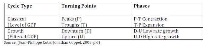
When analyzing the business cycles we use often use two approaches: first, the so called classical approach in which the turning points are selected on the basis of an absolute growth or decrease in GDP, and second, deviation or growth cycles where turning point are defined “with respect to deviations of the rate of growth of GDP from an appropriately defined trend rate of growth”. (Artis et all. 2002)
Table 1: A Taxonomy of Business Cycle Definitions
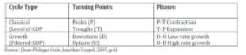
Once the turning points are known, the length of each cycle can be identified. In classical cycles, the period between the trough and the peak is the expansion phase and the period between the peak and the trough is the contraction phase. For a growth cycle, the upturn phase is defined as a period when the growth rate is above the long-term trend rate of growth and conversely for a growth downturn. (Jean-Philippe Cotis, Jonathan Coppel, 2005, p.6)
As a measure of economic fluctuations quarterly GDP indicator is most often used in the case of developed countries along with annual GNI. We will try through applying HP filter to extract the cyclical component for France.
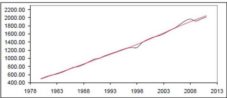
Fig 1. HP Trend France (1978-2013), Annual Data
Source: Our modelling based on OECD data (CQRSA: Millions of national currency, current prices, quarterly levels, seasonally adjusted)
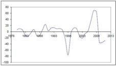
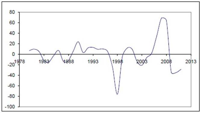
Fig 2. Business Cycles in France (1978-2013)
Source: Our modelling based on OECD data (CQRSA: Millions of national currency, current prices, quarterly levels, seasonally adjusted)
– CYCLE
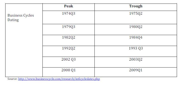
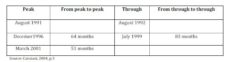
Table 2: Business Cycles Dating in France
In comparing the cyclical performance of countries like Germany and France it is necessary to underline the difference in their long — run performance. As we can see in the table, developed country like France is likely to have more recession due to its slow economic growth.
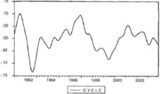
Fig 3. Business Cycles in Romania
Source: Caraiani, 2004, p.3
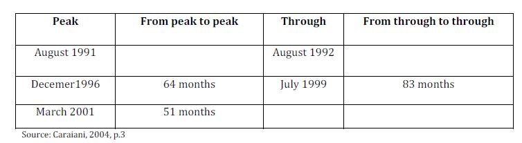
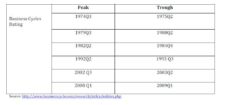
Table 3: Business Cycles Dating in Romania
Caraiani (2004) uses industrial production as main indicator in his analysis. In contrast to developed countries for Romania we found GDP data beginning only from 1997. Despite of this Caraiani solves the problem by directing his analysis only to the cyclical component. The finding thus obtained confirms the fact that the aggregate fluctuations in Romania are close to the ones found in developed countries. In Romania’s case our study relies on an analysis of three variables: growth in GDP, employment and industrial production. These indicators are interpreted below.
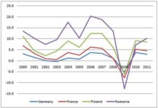
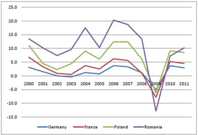
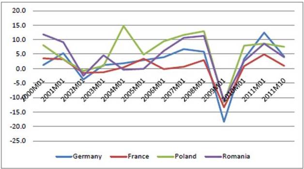
Fig 4. Growth in GDP
Source: Eurostat
We used the available data from Eurostat and shaped the graph in order to compare the dynamics of economical performance between developed and developing countries, members of UE. Despite the limits in expressing the real state of an economy, GDP is often used for this type of analysis. Keeping in mind that Poland became a UE member state in 2004 followed by Romania in 2007; both countries show some similarities with the overall trend shaped by the developed countries (Germany and France).
But there are also some interesting differences: for example, Germany and France had a period of economical contraction from Q3 2002 to Q2 2003 (Cotis and Coppel, 2005: 44), where Romania and Poland, in the same period, had an expansion phase after a turning point in 2002. The graph also shows differences in amplitude of fluctuations between contraction and expansion levels in the case of the two developing countries. For a well developed country the amplitude of the business cycle has declined (Cotis and Coppel, 2005: 13), which means that the economy is on a stable ground, with small rates of contraction and expansion and more prepared in moments of economical crises. In contrast, the growing economies are more fragile and more volatile which makes them more vulnerable in time of crises, despite the growth rates that they have in the so called economical boom times. As seen in the graph, the 2008 economical crisis affected all the economies, but Romania and Poland had much steeper drops in GDP compared to Germany and France.
After the peak moment found in august 2008, Romania had a dramatic decline in GDP volume compared with the previous periods due to a fall in investments and exports caused by changes in interest rates, which affected the credit (Caraiani, 2010: 135).
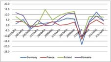
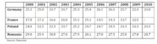
Fig 5. Industrial Production
Source: Eurostat
Industrial production is one of the main indicators used by Eurostat, OECD and other institutions for measuring business cycle dynamics. It provides a general measure of changes in the output volume in industrial, service and trade sectors of a national economy over a time period. Consequently, it shows both the nature and a health of an economy.
The moments of expansion and recession are also presented in this graph, seen around the year 2002 and 2008 respectively. Here we noticed that the much discussed crisis affected all countries studied translated by big drops around the year 2009 seen on the graph, with a slightly better performance in the case of France. Romania experienced a drop from 11.3% improvement over the same period in previous year to a -11.2% (and bellow) in 2009, followed by a strong recovery throughout 2009 and 2010, with a maximum reached in early 2011.
Table 4. Industrial Production Percentage in the Structure of GDP for Each of the Analysed Countries
Source: Eurostat
The industry has still a high contribution to regional GDP increased on average more than 20%, in countries like Germany, Poland and Romania. In Germany the industrial production increased with 2.6% reaching a level of 24% in the structure of GDP in 2010. In Poland and Romania, the industrial production increases with a lower percentage between 0.2-1.7 percent. In France the industrial production percentage in the structure of GDP have a relative low sore reaching a level of 12.5 percent in 2009. Nevertheless the industrial production in both developed and developing countries expanded at a more than 15 percent annualized rate (3m/3m, saar) toward the end of 2010. In 2011, according to the World Bank report, the industrial production began to slow in the first quarter of 2011.
Fig 6. Employment (Total Employment)
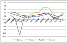
Source: Eurostat
Employment cycle is based on total employment series not seasonally adjusted expressed in percentage change compared to corresponding period of the previous year, based on inhabitants. Romania and Poland had a through point in first quarter of 2002, a point where both indicators presented above declined, describing thus a moment of contraction followed by another of expansion which consistently maintained until 2008, the year of the crisis. Germany and France show a slightly different trend with a light decrease in percentage until 2003 in case of Germany and the first quarter of 2004 for France. For the later the overall trend is quite constant with a small interval of fluctuations, in contrast with the former, developing countries. The explanations may differ from one case to another, but the consistency in the movement of all indicators in 2002 and 2008/2009 has some significance for assuming the presence of business cycles.
Conclusions
In a market economy the crises and recessions cannot be avoided. Consequently if we cannot get rid of them, then the problem should be reformulated: what can we do in order to limit the negative effects that appear naturally in these stages of the business cycle. From this point of view the approaches grow different from one another, but centred around two main guidelines. The first one speaks about stimuli groups for investments, direct investments and public expenses according to government policies. The second guideline gathers the proponents of the private initiative and of the laissez-faire that promotes the ‘private’ stimulation of the demand for investment and innovation.
Under crisis conditions the majority of the efforts at a macroeconomic level focus on the measures of fighting against it and on the possibilities to enter a new phase of the cycle, the recovery phase. In this context, a concerning aspect is the fact that in a crisis situation some states could place in the background their interest for sustainability, focusing on much pressing objectives, like the decrease in unemployment, inflation and the growth of the consumption disposition. Some investments in renewable energy based on the extensive use of manpower can build a strong stimulant for the short term and can maintain the sustainable character for the relation economy-environment, by reducing the emission of green house gases and by economic growth for the long term.
The cyclic phenomenon represents one of the key elements of the economic process that is the economy’s dynamics, because without it there is no possible balance for the economy. Its complexity “has stimulated the competition of the schools of thought” (Ţigănaș, 2003) enriching the economic science thanks to the variety of interpretations that they propose and bearing a smaller or greater ideological load. Thus it has influenced the science in the same manner as it has influenced the macroeconomical policies.
Acknowledgment
“This work was supported by the project “Post-Doctoral Studies in Economics: Training program for elite researchers – SPODE” co-funded from the European Social Fund through the Development of Human Resources Operational Program 2007-2013, contract no. POSDRU/89/1.5/S/61755.)”
“This work was supported by the the European Social Fund in Romania, under the responsibility of the Managing Authority for the Sectoral Operational Programme for Human Resources Development 2007-2013 [grant POSDRU/CPP 107/DMI 1.5/S/78342]”.
References:
Altug, S. & Bildirici, M. (2010). Business Cycles around the Globe: A Regime Switching Approach. International Business Cycle — Linkages, Differences and Implications, Budapest.
Publisher – Google Scholar
Artis, M. & Zhang, W. (1997). “International Business Cycles and the ERM: Is There a European Business Cycle?,”International Journal of Finance and Economics, 38, 1471-1487 York: National Bureau of Economic Research, 1946 [Online], [Retrieved December 22, 2011], http://www.businesscycle.com/research/intlcycledates.php
Publisher – Google Scholar
Baxter, M. & King, R. G. (1995). “Measuring Business-cycles: Approximate Band- Pass Filters for Economic Time Series,” Working Paper No. 5022, National Bureau of Economic Research.
Publisher – Google Scholar – British Library Direct
Benczur, P. & Ratfai, A. (2009). “Business Cycles around the Globe,” Manuscript.
Publisher – Google Scholar
Berger, H., de Haan, J. & Inklaar, R. (2002). ‘Restructuring the ECB,’ CESifo working paper no. 1084, Munich.
Burns, A. F. & Wesley C. M. (1946). ‘Measuring Business Cycles,’ New York: National Bureau of Economic Research, New York.
Google Scholar
Caraiani, P. (2010). “Modeling Business Cycles in The Romanian Economy Using The Markov Switching Approach,”Journal for Economic Forecasting, Institute for Economic Forecasting, vol. 0(1), 130-136, [Online], [Retrieved December 22, 2011], http://ideas.repec.org/a/rjr/romjef/vy2010i1p130-136.html
Publisher
Cotis, J. P. & Coppel, J. (2005). “Business Cycle Dynamics in OECD Countries: Evidence, Causes and Policy Implications,” The Changing Nature of the Business Cycle Reserve Bank of Australia Economic Conference, Sydney, Australia, RBA Annual Report, at http://ideas.repec.org/e/pco33.html
Publisher – Google Scholar
De Haan J., Inklaar R. & Jong-a-Pin R. (2005). “Will Business Cycles in the Euro Area Converge? A Critical Survey of Empirical Research,” University of Groningen, CCSO Centre for Economic Research, Working Paper, 08.
Publisher – Google Scholar
Festré, A. (2002a). “Money, Banking and Dynamics: Two Wicksellian routes from Mises to Hayek and Schumpeter,” The American Journal of Economics and Sociology, 61, 2, 439-480, [Online], [Retrieved May 13, 2011],http://halshs.archives-ouvertes.fr/docs/00/27/13/72/PDF/MOSS3.pdf
Publisher
Festré, A. (2002b). “Innovation and Business Cycles,” (in R. Arena and C. Dangel-Hagnauer (Ed.) “The Contribution of Joseph Schumpeter to Economics: Economic Development and Institutional Change”, 127-145), [Online], [Retrieved May 13, 2011], http://halshs.archives-ouvertes.fr/docs/00/27/13/62/PDF/Innovation_cycles_Schumpeter.pdf
Publisher
Furceri, D. & Karras, G. (2006). “Are the New EU Member States Ready for the EURO? A Comparison of Cost and Benefits,” Journal of Policy Modelling, 28, pp. 25-38.
Publisher – Google Scholar
Hayek, F. A. (1990). “Denationalisation of Money. The Argument Refined,” London, Institute of economic affairs, [Online], [Retrieved April 29, 2011], http://mises.org/books/denationalisation.pdf
Publisher
Keynes, J. M. (2009). ‘Teoria Generală a Ocupării Forţei de Muncă, a Dobânzii și a Banilor,’ Ed. Publica, București.
Google Scholar
Kurz, H. D. (2010). “The Beat of the Economic Heart Joseph Schumpeter and Arthur Spiethoff on Business Cycles,”MPRA Paper No. 20429, [Online], [Retrieved May 13, 2011], http://mpra.ub.uni-muenchen.de/20429/1/MPRA_paper_20429.pdf
Publisher
Lucas, R. E. (1977). Understanding Business Cycles, Stabilization of the Domestic and International Economy, Carnegie-Rochester Conference Series on Public Policy, Brunner, K. & Meltzer, A.H., vol. 5, Amsterdam: North-Holland.
Publisher – Google Scholar
Sargent, T. J. & Sims, C. A. (1977). ‘Business Cycle Modelling without Pretending to Have Too Much a Priori Economic Theory,’ Working Papers 55.
Savva, C. S., Neanidis K., C. & Osborn, D. R. (2007). “Business Cycle Synchronization of the Euro Area with the New and Negotiating Member Countries,” Centre for Growth and Business Cycle Research Discussion Paper Series No. 91.
Publisher – Google Scholar
Schumpeter, J. A. (1939). “Business Cycles. A Theoretical, Historical and Statistical Analysis of the Capitalist Process”, Ed. McGraw-Hill Book Company, New York, [Online], [Retrieved May 05, 2011],http://classiques.uqac.ca/classiques/Schumpeter_joseph/business_cycles/schumpeter_business_cycles.pdf
Publisher
Strand, J. & Toman, M. (2010). Green Stimulus, Economic Recovery, and Long-Term Sustainable Development, World Bank Policy Research Working Paper No. 5163.
Publisher – Google Scholar
Ţigănaș, C. (2004). “Ciclul Economic. Un Scurt Popas Doctrinar,” Analele știinţifice ale Universităţii Al. I. Cuza, Iași,Știinţe Economice, Tomul L/LI 98-106.
http://anale.feaa.uaic.ro/anale/resurse/13%20Tiganas%20C-Ciclul%20economic.%20Un%20scurt%20popas%20doctrinar.pdf.
Publisher