Introduction
One of the main phenomena observed in the process of stock returns is the presence of strong variations over times; these are periods of turbulence in financial markets. Statistically, the existence of these movements results in fat tails in the variations distribution function, calling into question the very strong assumption of Gaussian distribution returns. This empirical evidence has led to the invalidation of the famous formula of Black and Scholes (1973) that assumes that returns are generated from a normal distribution whose mean and variance are constant over time. Large efforts were then undertaken to consider the statistical properties of stock market fluctuations. The financial literature mainly concentrates on two approaches: the autoregressive models ARCH (Autoregressive Conditional Heteroscedasticity) introduced by Engel (1982) and the models with non deterministic volatility based on the works of Bachelier (1900). However, the big critic of ARCH model is a deterministic approach, while the other works consider making some volatility a random (unpredictable) variable. Several directions of research are developed for this approach: the stochastic volatility models introduced by Hull and White (1987), it is about a geometric Brownian process. It presents the major inconvenience not to be stationary. This type of specification was quickly abandoned for the benefit of the models generating a stationary volatility process, of type mean-reverting. Over time, the process tends to drift towards its long-term mean: such a process is named Ornstein-Uhlenbeck. Reference articles treating this type of model are the ones of Stein, E., and J.Stein (1991) for its simple version and of Harvey, Ruiz and Shephard (1994) for its logarithmic version. The econometric estimation of these models poses a challenge. Indeed, financial models are expressed in continuous time while observations can only be collected in a discrete time. On the other hand, the models studied are bivariate latent models where volatility is unobservable. First it is noticed that there is no analytical solution to this bivariate process. Therefore, we cannot consider exact discretization from which we could deduce a likelihood. The only way to cope with this is discretization approximation. Several discretization schemes are considered, the most popular being the Euler-method and the discretization ARCH. Volatility forecasting is an essential task in financial markets, so there are many papers that study forecasting performance of different volatility models in the literature, but many studies have been written in the theme of deterministic volatility modeling. The aim of this paper is to estimate and predict stochastic volatility from these two discretizations approaches above. Our empirical study is based on historical daily data of TUNINDEX in the period between December 31, 1997 and December 31, 2009. Unfortunately, there is no single procedure available to calculate and predict volatility. In this paper, the researchers compare the Kalman filter procedure (Harvey & al., 1994) and an EGARCH estimation approach (Nelson, 1990). The remainder of the paper is organized as follows. In section 2, there is a description of the estimation methods of the stochastic volatility model. Section 3 presents the forecasting Tunindex volatility. Section 5 concludes.
Estimating Stochastic Volatility TUNINDEX
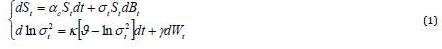
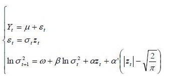
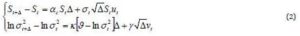
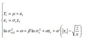
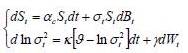
In this study, the logarithm of the instantaneous volatility follows the process of mean-reverting, also called the process “Ornstein-Uhlenbeck”. These reflect the presence of a force reverting to a long-term drift of the volatility. In particular, if S represents the value of TUNINDEX and if  symbolizes the logarithm of the instantaneous volatility, the dynamics of the bivariate diffusion process are governed by the following equations:
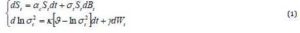
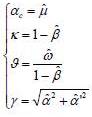
Brownian movement dBt and dWt are possibly correlated, E(dBt dWt)= Pdt .The coefficient P has a strong economic content because it represents the leverage effect. The parameters to estimate, for this type of model is the drift  , the long-term average
  , the speed of mean reversion K and volatility of volatility Y. These four parameters are considered constant, they will be determined from the database of the rate of return TUNINDEX between time t0 and T, which are respectively the first and last date in the database
Volatility Estimation via the Kalman Filter
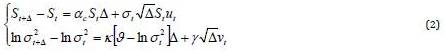
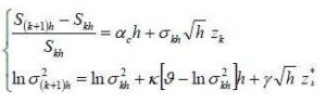
To estimate model (1), Harvey & al. (1994) conducted a linearization. This transformation helps to develop a model state measure. However, it should develop the log-OU by discretizing with a step equal to that of observations, denote by  the step of the discretization, for daily data, = 1/252 where approximately 252 is being the number of working days in a year, the discretization Euler gives:
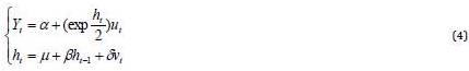
ut and vt , two error terms are Gaussian with zero mean and variance 1. This model can be rewritten as follows:
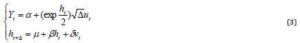
Yt indicates the return of the support  and
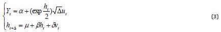
and  . Finally, the variations between two observations are modeled following the standard form:
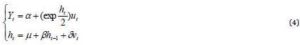
Formally adopting the notation Y = (Y1…YT) of the return vector of Support, h = (h1…hT) unobservable volatility vector and denote by  the set of parameters
  , the parameter
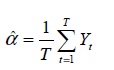
  must be estimated prior to effecting the linearization of the model. The estimator of is:
 (5)
(5)
To linearize the first equation of system (4), we square  and express it in logarithmic form. The following is obtained:
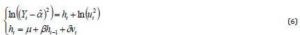
As further developing this equation as we know that ut ~ N (0.1), we can therefore deduce the distribution of In(ut2). It corresponds to a logarithmic χ2 distribution, whose expectation is -1.27 and the variance is 0.5  , approximately 4.93. Note however that In(ut2) cannot be correctly approximated by a normal law only if the sample is very large.
Following the approach of Racicot F.-E. and Theoret R. (2005), by adding and subtracting E In(ut2) in the first equation of model (6), we obtain:

Setting 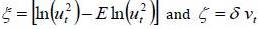 , we get two white noise centered on variance 4.93 and
  respectively.
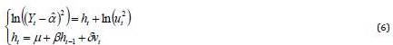
We can therefore rewrite the model (6) as follows:
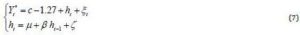
Where 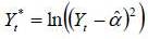 and c is a constant introduced to take into account that it equals only -1.27 in very large samples. This model is as state-space linear. Equations 1 and 3 of the model (7) are in the appropriate form to use the Kalman filter. The first equation is called measurement equation as the variable Y is observed. The second equation is the equation of state or transition as h the state variable is latent. The method of estimating this model is then explained in two steps: first, the latent variables are estimated by Kalman filter approach, then the parameters are estimated by the method of Maximum Likelihood.
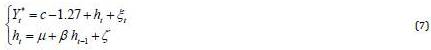
The researchers used EViews software for the implementation of this algorithm. The result of estimating the state-space model appears in the following table:
Table 1: Estimation of Stochastic Volatility of TUNINDEX Returns
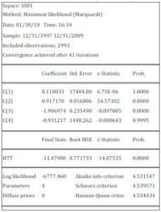
As obvious in Table (1), the coefficients C(1) and C(4) are not significant at the 95%. The coefficients C(1) to C(4) are the parameters of the model (7) with C(1)= c, C(2)=  and exp(C(3))= and C(4)=
  . Using the system of equations linking the parameters of discrete-time model with the parameters of the model in continuous time, table (2) is drawn to summarize the results of estimation for the log-OU after the Euler discretization. Note that the parameters obtained from this discretization are annualized.
Table 2 : Estimation Results for Log-OU Model
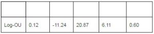
It is noted that the instantaneous volatility moves around a long-term trend equal to 0.45%. To achieve this, use the following equation  and take root. k relatively high value is also found, which suggests a pronounced effect of mean reversion.
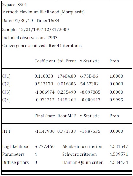
It is also noted that the coefficient of correlation P between movements in returns and movements in volatility is different to zero, which may justify the assumptions considered by some authors, such as Heston (1993) for example, who proved that the correlation between volatility and returns of assets is essential to generate the asymmetric distribution. The evolution of the observed variables and filtered of Y* illustrated in Figure (1)
 Figure 1: Values Observed and Filtred of
In option pricing models, volatilities are expressed yearly. In portfolio selection model in continuous time and for the calculation of VaR, the reference period is the day, volatility is expressed as daily. Moreover, according to the equation  , the stochastic volatility of TUNINDEX return is equal to:

To annualize this volatility, multiply  by
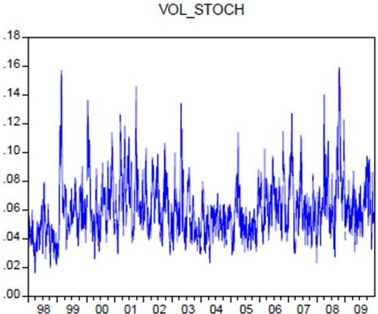
by  . In other words, the daily volatility is about 6% of annual volatility. The evolution of the volatility of TUNINDEX return is shown in figure (2).
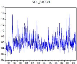
Figure 2: Stochastic Volatility of TUNINDEX Return
It is found that volatility is experiencing strong fluctuations around its average, which is 0.45% on daily basis, corresponding to 7.1% in annual frequency.
The first half of the decade was characterized by very high levels of volatility, the movement began in 1999, as shown in Figure (2), as a historical volatility. This period is also characterized by a multiplication of volatility peaks. A peak in volatility specifies a phase when the volatility settles at a level significantly above its long-term average. After a sharp drop between 2003 and 2005, the volatility has temporarily stabilized at a low level before increasing again in 2006. The increase in volatility during a period of time, results from a conjunction of proper phenomena to this period, such as the events of 11 September 2001, which significantly changed the aspect of risk taking behavior of investors just like the aspects of growth.
Exponential Model of Autoregressive Conditional Heteroscedastisity
Models of the ARCH family (Autoregressive Conditional Heteroscedasticity) have enjoyed considerable success since their first version put forward by Engel (1982). Nelson (1990) showed that ARCH models have the same stationary distributions that some stochastic volatility models expressed in continuous time. Specifically, the E-GARCH model has the same stationary distribution as a version of log-OU given by model (1). Indeed, this model is very useful to model not only excess kurtosis but also asymmetric effects that have returns on volatility. The simplest and most used EGARCH model is the EGARCH (1,1) defined as follows:
Where Yt is a random variable representing the arithmetic return of the support St, Zt  N(0,1) and
  are real constants.
The process  is AR (1) and admits a stationary solution if and only if
  .
.
Resume model (1):
Where E(dBt dWt)= Pdt.
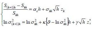
Nelson (1990) proposes a suite of models indexed by h which converges in distribution to model (1), when the amplitude of the elementary time interval approaches zero. Consider the family of models:
Where 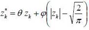 . Indeed the two random variables: Zk and
  are centered, reduced and uncorrelated. The parameter allows to model the asymmetric effect related to the sign of innovation Zk and the parameter
  takes into account the asymmetry related to the amplitude of innovation Zk as measured by the difference
  .
.
Therefore, the EGARCH model (1.1) describes a mean-reverting process. So the logarithmic conditional variance returns in long-term  with speed K . The researchers will apply this model to Tunindex return in the period between December 31, 1997 and December 31, 2009. Table (3) represents the results of estimating EGARCH (1,1) model.
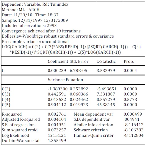
Table 3- Estimation of Conditional Volatility of Tunindex Returns
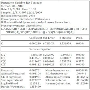
As can be seen from the table above, the coefficients C, C(2), C(3) and C(5) are significant at the 95%. The coefficients C, C(2), C(3), C(4) and C(5) are respectively the parameters  of the EGARCH (1.1) model.
After estimating the EGARCH (1.1) model with maximum likelihood method, the parameters of the model (1) can be determined by the following equivalence:
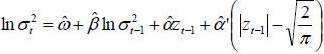
From EGARCH (1,1) model, an estimate of the conditional volatility can be proposed, according to the equation:
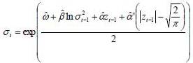
 indicate the maximum likelihood estimating.
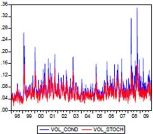
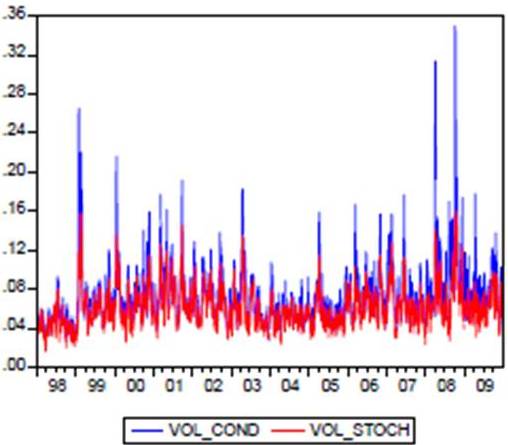
Figure 3: Stochastic Volatility and Conditional Volatility of Tunindex Returns
In Figure (3), we compare the conditional volatility associated with the EGARCH (1.1) model to stochastic volatility calculated previously. It is noted that the profiles of evolution of the two volatility curves are very close. We also observe that the stochastic volatility fluctuates less than the conditional volatility. In this case, the conditional volatility associated with the EGARCH (1,1) model had increased further during the market crash of October 2008.In this study, the leverage effect is represented by ; it is positive and statistically different from zero. In figure (4), the new impact for Tunindex return by NIC (News Impact Curve) is determined; the curve representing the variance  against impact
Which.
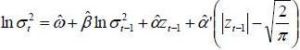
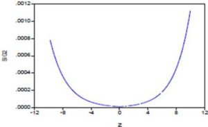 Figure 4: News Impact Curve of Tunindex Return
An asymmetric leverage effect is clearly observed in Figure (4). Thus, the conditional variance of Tunindex return reacted more to positive shocks than negative shocks of equal magnitude. The economic consequence of this result is that an unanticipated increase in Tunindex return leads to increased uncertainty greater than that induced by an unanticipated drop in return.
Forecasting TUNINDEX Volatility
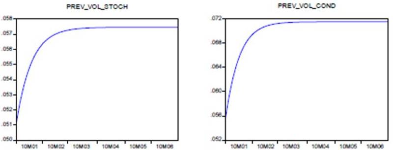
It is now possible to produce forecasts of volatility from the models established, which are strictly recursive. Take the case of TUNINDEX. The forecast starts January 02, 2010, the sample ending on the date of December 31, 2009, and we continue to forecast until June 30, 2010. The result of forecast is shown in Figure (5). As can be seen, the stochastic volatility model provides an increase in volatility like the EGARCH (1,1) model. But it should be noted that the volatility arising from the EGARCH (1.1) model was initially slightly higher than the stochastic volatility. Thus, the two volatilities tend to be closer to their equilibrium value in the long term.
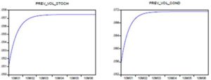
Figure 5: Forecasting Tunindex Volatility: Kalman Filter Model and EGARCH (1,1) Model
To explore the robustness of forecast accuracy, the root mean squared forecast error or RMSFE criterion was employed.
Applying this formula:
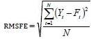
Where Yt is the actual value at period t, and Ft is the forecast for period t. Hence, RMSFE based on Kalman filter forecast model is lower than the one based on EGARCH forecast model. That is why we strongly recommend the Kalman filter as a powerful tool to forecast stochastic volatility.
Conclusion
In this paper, the researchers demonstrate their interest in stochastic volatility model where volatility is governed by logarithmic Ornstein-Uhlenbeck process. This specification has been frequently used in the literature to describe the volatility process, mainly because of its convenience and simplicity.
The estimation procedures associated are the state-space model and the EGARCH(1,1) model. Our empirical study is based on the historical daily data of TUNINDEX in the period between 31 December 31, 1997 and December 31, 2009.
This wide research reflects the importance of volatility in investment. So the empirical results have confirmed the hypothesis of correlation between movements in Tunindex returns and movements in volatility. In fact, an unanticipated increase in Tunindex return leads to increased uncertainty greater than that induced by an unanticipated drop in return. In addition, estimates obtained from the two discretization schemes (Euler and ARCH) are quite similar.
Forecasting the returns volatility, regardless of the model used, is an exercise fraught with risk. The model of stochastic volatility predicted an increase in volatility like the EGARCH (1, 1) model. But it should be noted that the volatility arising from the EGARCH (1, 1) model was initially slightly higher than the stochastic volatility. Thus, the two volatilities tend to be closer to their equilibrium value in the long term.
This survey has concentrated on the question: which method will provide the best forecasts? Forecasting can be a tedious task for financial analysts because of discrepancies in the results provided by different tools. The researchers strongly recommend the Kalman filter as a powerful tool to forecast stochastic volatility. However, both models remain easily implementable alternatives to more complex and computer-intensive techniques such as MCMC.
A good forecast of the volatility of asset prices over the investment holding period is a good starting point for assessing investment risk. Thus, volatility forecasting will continue to remain a specialist subject and will continue to be studied vigorously.
(adsbygoogle = window.adsbygoogle || []).push({});
References
Ait-Sahalia, Y. & Kimmel, R. (2007). “Maximum Likelihood Estimation of Stochastic Volatility Models,” Journal of Financial Economics, 83, 413–452.
Publisher – Google Scholar – British Library Direct
Andersen, T. & Lund, J. (1997). “Estimating Continuous-Time Stochastic Volatility Models of the Short-Term Interest Rate,” Journal of Econometrics, 77, 343-377.
Publisher – Google Scholar – British Library Direct
Bakshi, G., Cao, C. & Chen, Z. (1997). “Empirical Performance of Alternative Pricing Models,” Journal of Finance, 52, 499-547.
Publisher – Google Scholar – British Library Direct
Broto, C. & Ruiz, E. (2002). “Estimation Methods for Stochastic Volatility Models: A Survey,” Universidad Carlos III de Madrid, working Paper, (14), 02-54.
Publisher – Google Scholar
Dempster, A. P., Laird, N. M. & Rubin, D. B. (1977). “Maximum Likelihood for Incomplete Data via the EM Algorithm,” Journal of the Royal Statistical Society B(39), 1-38.
Publisher
Ferland, R. & Lalancette, S., (2006). “Dynamics of Realized Volatilities and Correlations: An Empirical Study,” Journal of Banking & Finance ,30, 2109–2130.
Publisher – Google Scholar
Figlewski, S. (1997). “Forecasting Volatility,” Financial Markets, Institutions and Instruments , 6(2).
Publisher – Google Scholar – British Library Direct
Fornari, F. & Antonio Mele, A. (2006). “Approximating Volatility Diffusions with CEV-ARCH Models,” Journal of Economic Dynamics & Control , 30, 931–966.
Publisher – Google Scholar
Gelfand, A. & Smith, A. (1990). “Sampling-Based Approaches to Calculating Marginal Densities,” Journal of the American Statistical Association, 85, 398-409.
Publisher – Google Scholar
Mills, T. C. (1995). “Modelling Skewness and Kurtosis in the London Stock Exchange FT-SE Index Return Distributions,” The Statistician, 44(3), 323–332.
Publisher – Google Scholar
Peiro, A. (1999). “Skewness in Financial Returns,” Journal of Banking and Finance, 23, 847–862.
Publisher – Google Scholar
Saatcioglu, C., Levent Korap, H. & Volkan, G. (2007). “Information Content of Exchange Rate Volatility: Turkish Experience,” International Business & Economics Research Journal, (6), 9-14.
Publisher – Google Scholar – British Library Direct
Shinichi, A. & Bagchi, A. (2006). “Filtering and Identification of Heston’s Stochastic Volatility Model and its Market Risk,” Journal of Economic Dynamics & Control ,30, 2363–2388.
Publisher – Google Scholar