Introduction

Financial market facilitates channeling of capital from segments with its surplus to deficit and matches counterparties with the intention of an efficient investment. Bodie, Kane and Marcus (2021) highlighted that either individual or institutional investors commit their capital to selected investment opportunities and anticipate adequate benefit which is a satisfactory rate of return from their unique allocation. For that reason, within the investment analysis the essential analytical task is to determine portfolio proportions subjected to individual objectives. Markowitz (1952) proposed a quantitative framework that aims at defining a portfolio formulation procedure in which, taking into account portfolio statistics, investment participants at all times prefer higher rates of return whilst exposed to a certain risk level or, correspondingly, for a particular expected rate of return they always favor lower extent of volatility. Bali and Peng (2006), Lundblad (2007) or Lettau and Ludvigson (2010) confirmed that there is a statistically significant positive trade-off between financial instruments expected rates of return and volatility, as well as Aliber (2011) emphasised that if market turbulence is present, either as a result of systemic or idiosyncratic risk materialisation, an increase in the volatility of market parameters and, consequently, financial instruments valuations are also observed. Formally, the riskier a financial instrument is, or the higher its potential loss, the higher its expected rate of return, whereas the collective investment portfolio is characterized with a lower risk level than a sum of risks of individual assets. The cited rationale is considered as the fundamental notion of the portfolio theory (as reminded in, e.g. Elton et al. (2014)). Thus, it is true that the optimal portfolio holds a combination of financial instruments with the possibly best risk-return trade-off.

Due to the recent wave of investment losses related to the aftermath of the SARS-CoV-2 pandemic the significance of portfolio risk management was again revealed. In the wake of a financial crisis correlations of securities’ rates of return use to highly appreciate and differ from these implied by the economic fundamentals what was scrutinized for financial market collapses by Loretan and English (2000), Hartmann, Straetmans and de Vries (2004) and Bekaert, Campbell and Ng (2005) and identified as a contagion phenomena. Goetzmann and Kumar (2001) further emphasise that it may, e.g. influence the efficiency of the idiosyncratic risk diversification effect and require pro cyclical portfolio rebalancing. Consequently, more robust asset selection strategies are elaborated and it remains crucial to apply a competent optimisation technique for a rational investment decision-making which assures of anticipated risk-return trade-off.

Therefore, in this paper, a portfolio formulation procedure is developed to enhance the efficiency of assigning proportions to selected securities under the modified Markowitz’s framework with the use of sampling methods and genetic algorithms at increased market volatility. Firstly, the model is based on an assumption presented in Litzenberger and Modest (2008) that financial market is mostly quiescent (business-as-usual/non-crisis; low market volatility) and is infrequently interrupted by stress (crisis; high market volatility) time periods. Secondly, it minimizes the negative effects of identified market volatility relation between both quiescent and stress instances in order to reduce the necessity of, e.g. investment position rebalancing what, ceteris paribus, limits the related transaction costs. Additionally, the attribution of the portfolio proportions is done using genetic algorithms (i.e. a probabilistic search engine used in, e.g. machine learning, first introduced by Holland (1975), which emulate operations from natural selection mechanisms based on the survival-of-the-fittest principle) for sampled input data, either from empirical distribution or a theoretical distribution. All to address the estimation risk problem which is related to potentially biased historical input data examined by Orwat-Acedańska and Acedański (2013). Similarly formulated investment portfolios may be regarded as an addition to literature and also serve as an alternative to commonly utilized mean-variance optimization techniques.

Thus, this paper intends to resolve the research question whether the adoption of the abovementioned portfolio formulation procedure and optimization tools by an individual or an institutional investor could improve the efficiency of securities allocation, distinctively, at an increased market volatility, e.g. stemming from exogenous events.

The remainder of this paper is organised as follows. In Chapter 2 a formulation of the market volatility-robust investment portfolio composition approach under the modified Markowitz’s framework with the use of sampling methods and genetic algorithms was outlined. Next, in Chapter 3 research findings were provided based on the empirical example of an investment portfolio optimization with an use of the developed approach. Afterwards, in Chapter 4 a dedicated portfolio backtesting was done. Finally, conclusions were stated.

The model

Portfolio theory background

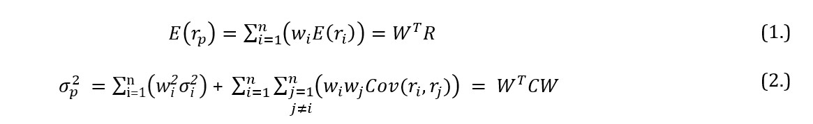
Markowitz (1959) assumed that securities rates of return follow the multivariate normal distribution which implies that an investment portfolio is described by its expected rate of return E(r_p) and variance  such as:

where W is a matrix of proportions w_i (attributed to i-th security), R is a matrix of expected rates of return of selected financial instruments and C is their symmetric variance-covariance matrix.

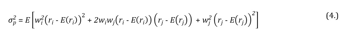
In line with the above, the rate of return of a formulated portfolio is always a weighted average of rates of return of its comprising financial instruments and, simultaneously, is the basic measure of the average yield from the investment. The variance of a formulated portfolio, however, is not the weighted average of the separate securities variances. In case of an investment portfolio built upon two financial instruments the inherent risk is understood as:

where  is the two asset portfolio variance, w_i and w_j are the weights attributed to securities i and j, r_i and r_j are the rates of return of the securities i and j, whereas E(r_i) and E(r_j) are their expected values. Application of the binomial theorem, i.e. , reduces the variance of two financial instruments portfolio to the form of:

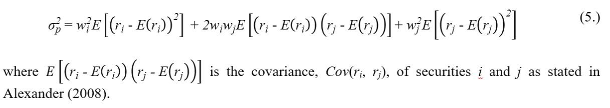
from where it is useful to recall the properties of the expected value statistic. If the mean of a sum of two rates of return is equal to the sum of mean of each rates of return (i.e. ) and if a mean of constant multiplied by the rate of return is equal to the product of the constant and the mean of the rate of return (i.e. ) it is true that:

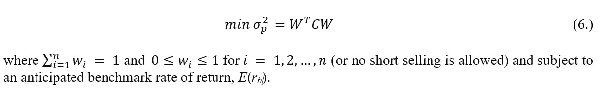
As provided in Merton (1972), Elton and Gruber (1977) and reminded in Bodie, Kane and Marcus (2021) there are two plausible approaches for either individual or institutional investors with a single period portfolio formulation problem to consider. First, (a.) to minimise the volatility of an investment portfolio for a given expected rate of return which results in finding the solution to an optimisation problem with continuous random variables, quadratic objective and linear constraints. Second, (b.) to maximise the expected rate of return of an investment portfolio for a given volatility which involves solving an optimisation problem with continuous random variables, however, with a linear objective and all linear constraints but one quadratic limitation. Woodside-Oriakhi, Lucas and Beasley (2011) pointed that even though both methods resemble logically one another, approach (a.) is computationally more efficient. Subsequently, the portfolio optimisation problem is often defined as:

Sampled market volatility-robust investment portfolio

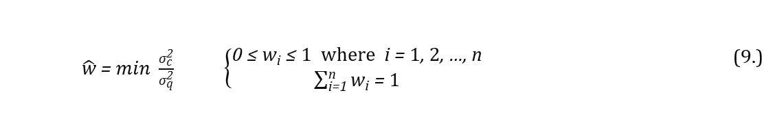
If the assumption is implemented that financial market is mostly quiescent (volatility-wise) and is infrequently interspersed with exogenous stress periods, either individual or institutional investors consider the possibility of relevant decline in the rates of return on financial instruments and increase of volatility as mentioned in, e.g. Kole, Koedijk and Verbeek (2006). In that manner, to obtain a volatility-robust investment portfolio the formulation procedure shall minimise the quotient of variances in both quiescent  and stress periods  formulated as:

where C_q and C_c are symmetric variance-covariance matrices for respectively quiescent and stress intervals. In addition, w_i are the proportions of capital allocated in i-th security under either quiescent or stress regime (with no short selling) which sum up to 1. As such, the optimisation problem is defined as:

Intrinsically, the market volatility-robust investment portfolios allow for less frequent position rebalancing which diminishes inherent transaction costs (especially transaction fees but also other operational costs) and what might be attractive for passive investment strategists that seek to reduce the consequences of increased market volatility on their allocation.

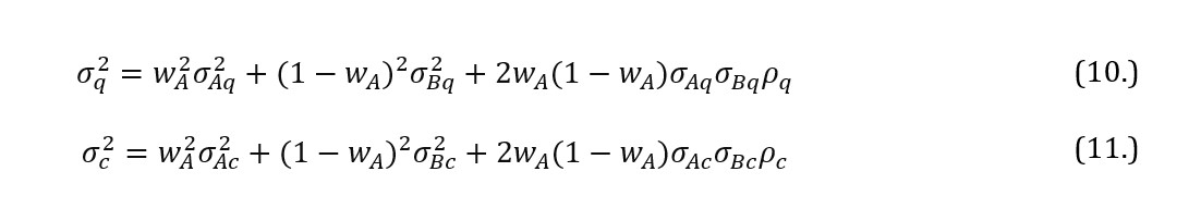
Analytically, in case of a two financial instruments portfolio, if variance in quiescent period is  and in time of market stress is , correlation coefficient of securities rates of return is  (during non-crisis interval) and  (in crisis) and short selling is not allowed (  where w_i ∈ ), then the portfolio formulated of two financial instruments is built of proportions w_A for instrument A and (1 – w_A) for instrument B. As a result, it is true that

To extract the proportion w_A that minimises  , it is necessary to differentiate with respect to w_A which results in:

If the correlation coefficient of financial instruments rates of return in quiescent period is a lower value then its equivalent in stress period (or   > ) then the contagion phenomena is revealed. Otherwise (i.e. < ) a flight-to-quality effect when volatility increases while correlation between selected instruments decreases as described in Baur and Lucey (2009). Importantly, the analysis and implementation of the latter might provide an opportunity to formulate as stress-insensitive investment portfolio as possible. In essence, when the flight-to-quality effect is observed the correlation spread between the quiescent and stress intervals is negative, what allows to obtain a satisfactory volatility and correlation trade-off. Therefore, if  is not equal to one it means that correlations of financial instruments rates of return differ in stress periods, the proportions condition may be simplified to:

for the market volatility-robust portfolio composition. The suggested framework seems applicable for all asset classes, provided that the quiescent/stress regime is assumed and model input data is segregated accordingly.

Moreover, in the Markowitz’s framework the proportions  are found based on observations of financial instruments rates of return from a single sample what might cause estimation bias, especially, if data is characterised with statistical outliers or rates of return are asymmetrically distributed. Eventually, estimation risk materialisation results in suboptimal allocation. In this manner, sampling methods are used to overcome the unfavorable outcome of identified estimation risk. In this paper, many input data samples are drawn either from an empirical distribution or a theoretical distribution in order to minimise the risk of not receiving an optimal solution to the investment portfolio optimization task. Thus, the results are an average of proportions w_i derived from multiple scenarios. Michaud (1998) pioneered this technique for asset allocation. Orwat-Acedańska and Acedański (2013) summarised that mostly the phases of a portfolio formulation procedure in accordance with the Michaud’s sampling methods approach are as follows:

• Based on an initial sample – (k x n) matrix of rates of return observations – a l-amount of subsamples of the same size as the initial sample is extracted. Subsamples may be taken from either an empirical distribution (bootstrapping methods) or from a theoretical distribution (Monte Carlo simulations).
• For each subsample j (j = 1, 2, … , n) an estimation of [optionally a E(r_j) vector and] C_j (variance-covariance) matrix is done.

• [Optionally for defined minimal benchmark rate of return E(r_b)] Proportions w_j are attributed.
• Subsample j investment portfolio proportions are averaged:

Scherer (2002) highlighted that, in comparison to the Markowitz framework (i.e. to mean-variance optimisation), the allocation performed in the above manner is more diversified and is less susceptible to radical alterations often needed at an increased market volatility. Also, sampling methods may be used for a wide variety of financial instruments rates of return distributions and for risk measures other than variance, e.g. coherent CVaR. In this paper, the discussed methodology is further enhanced with the use of genetic algorithms as an optimisation technique (and alternative to Newton’s method) which is independent of adopted objective function and might be adjusted to real rates of return distributions as stated in Chang et al. (2000).

Genetic algorithms framework

Genetic algorithm’s framework is classified as a subcategory of evolutionary algorithms where the prime objective of a computation process is to emulate operations directly from the Darwinian natural selection which follows the survival-of-the-fittest principle as described in books, e.g. Goldberg (1989) or Michalewicz (1996). Following, Engelbrecht (2007) provides that chromosomes (or individuals c_i) are grouped in a population in which a gene g_i is an exclusive characteristic of a chromosome and an allele a_i is the gene’s value. In specific, genetic algorithms seek an optimal solution via population manipulation which size does not change throughout iterations (or generations) of possible outcomes. Mitchell (1999) emphasizes that a typical algorithm follows three steps. First, a population of individuals has to be established. Second, the selection of adequate chromosomes has to match the best fitness function value criterion. Third, for a creation of next generations, the crossover process is compulsory and solutions shall mutate.

Chromosomes that are meant to survive until next iterations are evaluated in terms of their fitness function values f. Thus, an evaluation operator is intended to attribute a grade to an individual outcome in respect to its measure of fitness. Subsequently, with the use of a selection operator, as stated in Yang (2006), the population structures that are characterized with higher fitness function values are duplicated, whereas population structures that are marked with lower fitness function values are rejected. Whitley (2001) concludes that simply the fitter individual the more likely it survives and forms a set for further iteration.

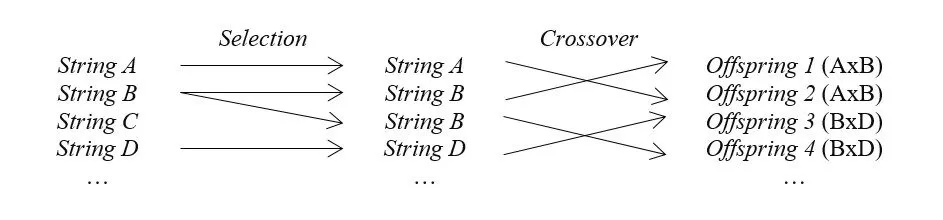
In order to derive a new individual (offspring, o_i), the crossover operator matches selected parents at a crossover point, as explained in Schmitt (2001). Therefore, every prospective result incorporates properties of the previously picked chromosome pair, though, is different from the starting generation. Finally, entire procedure is replicated and another pool of solutions with a satisfactory value of fitness function crossover to produce next generation is obtained. Figure 1. is a graphical illustration of the phases of construction of a new generation of chromosomes.

 Figure 1: Construction of a new generation of chromosomes

Source: Own elaboration.

All additional alternations are made within the individuals with the use of mutation operator. Random changes are slight and plausible to occur in all genes. Consequently, different set of potential candidates that are gained from original chromosomes is calculated.

Iterations proceed until the algorithm reveals no improvement in solutions fitness function value. It is apparent information that an optimal outcome is approached. Otherwise, the process continues to fixed termination criterion fulfilment. Kumar et al. (2010) emphasise that termination conditions are mostly met if, e.g. an early acceptable solution is obtained, a shortage of funds or time is observed, a predetermined number of iterations is done, or iterations do not provide any additional information value.

Selection operator

All selection operators are attributed to selection pressure. Goldberg and Deb (1991) and Bäck (1994) relate selection pressure to time interval from the beginning of a genetic algorithm’s exploration until the point in which an uniform population is produced. If selection pressure is recognized at a too low level than genetic algorithms convergence rate is too low in terms of an optimal result. Conversely, if selection pressure is recognised at a too high level, than the population is devoid of required diversity.

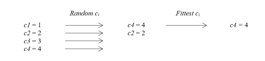
Thus, in this paper, a tournament selection is used where a random pool of chromosomes is separated from the total population. Next, the group is evaluated in terms of fitness function values and prime individual is allowed to crossover as stated in Pereira (2000). Whole process is repeated n-times to fill the mating pool. Formally, in tournament selection the selection probability p_s of an individual ready to reproduce is defined as:

where m is the extracted set of chromosomes. In case when separated tournament is not of considerable size in comparison to population, selection algorithm does not allow the fittest individual to dominate. However, as referred in Razali and Geraghty (2011) if the detached group is heavily undersized in regard to population, it is more likely that inadequate outcomes will be selected. Figure 2. depicts a tournament selection mechanism.

 Figure 2. Tournament selection method

Source: Own elaboration.

Crossover operator

Throughout crossover the selected individuals blend information they carry (from previous generations). Spears and Anand (1991) noticed that for larger populations’ crossover process assures that genetic algorithms avoid random decisions and outputs are precisely pursued into anticipated range of solutions. Selection mechanisms draw appropriate chromosomes out of the population. However, it is important to control if newly created offspring is not an exact copy of its predecessors. This may indicate that one individual was set to a role of two parents. Similar operations should be limited to enhance the algorithm’s computation performance.

In that manner, in this paper, a two-point crossover operator is used where parental individuals are partitioned in two randomly specified break points. Therefore, three segments are obtained accordingly. Hasancebi and Erbatur (2000) state that the gene replacement procedure is completed by a swap of either outside segments or inner part of a chromosome. It is useful to notice that regardless of an exchanged gene sequence the final solution will be identical. For best illustration two chromosomes encoded such as c₁ = [1 1 0 0 1 0 1 0] and c₂ = [0 1 1 0 1 1 0 0] are considered. Two-point crossover break points are randomly set. First segmentation is done after the second gene and second segmentation is done after the third gene in both parental individuals bit strings. So that sub-vectors are as follows:

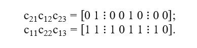
In a reproduction procedure, outer sections are exchanged. Sub-vector c₁₁ swaps with c₂₁ and c₁₃ with c₂₃ such as:

Consequently, next generation of chromosomes is attained, precisely o₁ = [0 1 0 0 1 0 0 0] and o₂ = [1 1 1 0 1 1 1 0]. Bäck (1996) stresses that a two-point crossover method is more likely to preserve top genes until next iteration, in comparison to popular single point crossover, and it could be extended to N-point reproduction.

Mutation Operator

Mutation operator is implemented to retain diversity of a population. In particular, a genetic algorithm uses mutation to omit early convergence to a local optimum and to refrain from premature solutions. Mutation probability p_m is usually a constant value what implies that all chromosomes are equally likely to mutate, regardless of their assigned fitness function values. However, Marsili-Libelli and Alba (2000) noted that it is more efficient to adopt a mutation operator which is a function of fitness. Typically, an adaptive mutation operator identifies lower evaluated genes in highly fit individuals and afterwards improves their accuracy, whereas chromosomes with relatively smaller fitness function values hold increased likelihood of mutation, so that their role in population is enhanced.

Therefore, in this paper, if  is an average fitness function value of a population and a chromosome is characterized with fitness f then mutation probability is considered in two cases. If  > f, mutation probability is kept random. If  < f solution encoded in a chromosome is good enough to lower mutation probability to avoid schema disruption.

Research Findings

Input data

In order to verify the practicality of the suggested approach, an investment in 10, diversified-by-sectors WIG20 traded blue-chip securities, i.e. CDR (gaming), CPS (telecommunication), KGH (metal extracting and production), LPP (clothing), PEO (banking), PGN (gas extraction and energy), PKN (crude oil extraction and production), PKO (banking), PZU (insurance) and SPL (banking) was assessed.

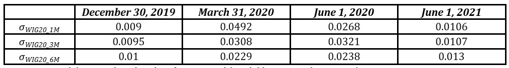
Firstly, logarithmic rates of return were calculated based on historical daily prices of the above-mentioned securities for the trading days from January 1, 2015 until June 1, 2021 (1 602 publicly available observations). Next, a risk benchmark was defined (i.e. WIG20 volatility) where it was assumed that the volatility (measured as standard deviation) of the risk benchmark  should be calculated for at least three moving time intervals (i.e. 1M, 3M, and 6M). It was further adopted that if  for the shortest-term interval was a higher value than for the medium-term interval and longer-term interval, and if volatility for the medium-term interval was a higher value than longer-term interval (i.e.  then a stress period, or simply a crisis was identified. The input data was segregated accordingly and assigned to subsamples q – quiescent and c – stress. Further, to solve the optimization problem stated in the formula (9.) a genetic algorithm that utilises tournament selection, two point crossover and adaptive mutation operators was employed. The initial population size was settled at 100 chromosomes and entire procedure lasted for 500 generations – the adopted termination criterion regularly stopped the genetic algorithm after 500 iterations (given an optimal solution was not received earlier). The allocation was performed for the end of 2019 (December 30, 2019) and further backtested at three moments, i.e. March 31, 2020, June 1, 2020 and June 1, 2021 where the latter dates included market conditions  related to SARS-CoV-2 pandemic influence on financial markets (increased volatility; Table 1.).

Table 1: Risk benchmark volatility at December 30, 2019, March 31, 2020, June 1, 2020 and June 1, 2021

Source: Own elaboration based on data from stooq.pl (available at November 1, 2021).

Also, once the input data was segregated for both periods subsamples q and c, another data subsamples were drawn with replacement with the use of sampling methods either from an empirical distribution (bootstrapping methods) or a theoretical distribution (Monte Carlo simulations). Next, the symmetric variance-covariance matrices C_q and C_c were constructed. Ultimately, the allocation was performed via minimization of the data subsamples c and q volatilities quotient with the use of defined genetic algorithms as an optimisation tool. The final results (i.e. portfolios) were an average of proportions and statistics obtained from 1 000 formulation procedures as stated in Chapter 2. In the end, the received allocations were compared to proportions and portfolio statistics received with a classic Markowitz’s framework.

Empirical results and analysis

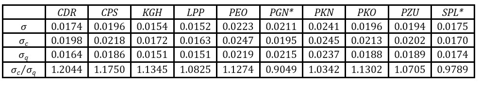
Baseline investment portfolio was formulated for the end of 2019 (December 30, 2019). It means that the input data included 1 247 logarithmic rates of return for corresponding trading day observations (starting from January 1, 2015). In line with the risk benchmark volatility criterion (i.e. ) the initial input data was segregated into subsamples q and c (with 327 and 794 trading days observations respectively) and was characterised by individual securities volatilities as presented in Table 2.

Table 2: Segregated data volatilities at December 30, 2019p

* Naturally, noted volatilities within the c data set were anticipated to be higher in value than their counterparts in q. Nonetheless, such relation was not observed for PGN and SPL which, ceteris paribus, in relatively stable market conditions at Warsaw Stock Exchange remained more unexpected with more volatile rates of return.

Source: Own elaboration based on data from stooq.pl (available at November 1, 2021).

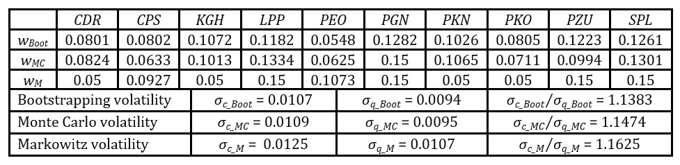
Next, out of initially segregated input data subsamples q and c, sampled data sets were further generated with both bootstrapping methods and Monte Carlo simulations. For newly obtained data sets corresponding C_q and C_c matrices were calculated. As such, 1 000 optimisations were performed for constraints that included also no short selling. The results from iterations were afterwards averaged to finally obtain the minimal value of the quotient of data subsamples c and q volatilities. Complementary, the Markowitz allocation was done for comparison. A summary of the optimised portfolio proportions and volatility statistics are included in Table 3.

Table 3. Optimised portfolio proportions and volatility statistics at December 30, 2019 

Source: Own elaboration based on data from stooq.pl (available at November 1, 2021).

Thus, consistent for all considered allocations in comparison to Markowitz framework, firstly, the portfolio formulation procedure utilising sampling methods and genetic algorithms provided more diversified portfolios (i.e. with lower concentration). Secondly, the averaged volatilities for both subsamples q and c were lower and their lower quotients were observed. Also, mostly a flight-to-quality effect was observed for the considered averaged correlation spreads between subsamples q and c.

Backtesting

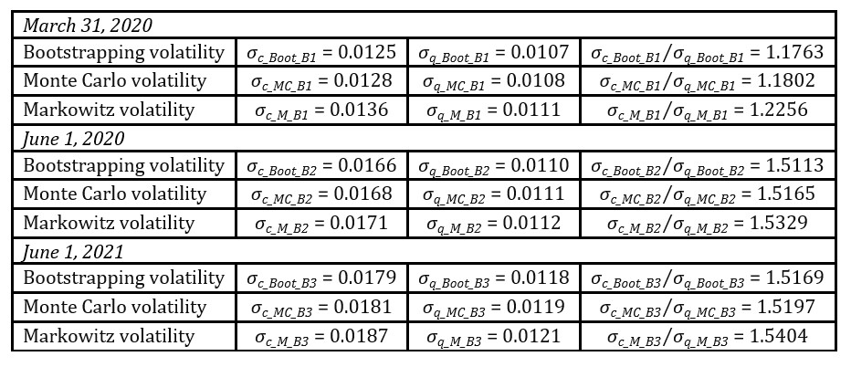
In order to verify if historically obtained market volatility-robust portfolios reduced the necessity of investment position rebalancing (to lower transaction costs) in following time periods an allocation backtesting was done. In that manner, optimised proportions analysed at the end of 2019 were exchanged for their next time period counterparts. A summary of backtesting volatility calculations is presented in Table 4.

Table 4. Allocation backtesting and volatility statistics at March 31, 2020, June 1, 2020 and June 1, 2021 

Source: Own elaboration based on data from stooq.pl (available at November 1, 2021).

Having all things considered, it was observed that the suggested approach efficiently minimises the unfavourable effects of an increased market volatility in an investment portfolio formulation problem by providing less risky portfolios. Therefore, it seems that, surprisingly, not enough attention is paid in the literature to the use of multiple scenario analysis in solving the portfolio formulation problem

Conclusions

In this paper, a model under the modified Markowitz’s approach with the use of sampling methods and genetic algorithms was developed to improve the efficiency of allocation in a portfolio formulation procedure at an increased market volatility. The suggested approach contributes to the existing methods of limiting the risk of not receiving optimal solutions in security allocations. Also, the research adds a rationale for the developed quantitative framework to be included in the literature and to practical use either in individual or institutional investor strategies.

In reference to the obtained computational results, it was observed that, firstly, in order to obtain a more diversified investment portfolio, it is important to overcome the limitations of a single sample analysis that may be biased, especially, due to statistical properties of expectations of rates of return (e.g. if outliers are observed or rates of return are asymmetrically distributed). Therefore, a portfolio formulation procedure with the use of sampling methods and genetic algorithms as an optimisation tool was proved to provide a less concentrated allocation in comparison to, e.g. Newton’s method, used for optimization under Markowitz’s framework. Secondly, the analysed averaged volatilities values for both subsamples q and c, pertaining to market instances, were lower what resulted in their lower quotient and imply that investment portfolios formulated with the use of multiple samples derived either from an empirical distribution or a theoretical distribution are less risky. In the end, all of the above enhance the investment decision-making process.

At present, however, this paper puts emphasis on model verification based on input data on WIG20 blue-chip securities so that all market parameters are local. Because of that, further research is required, inter alia, to ascertain if similar conclusions were directly applicable to other jurisdictions and, importantly, to different asset classes. Moreover, since sampling methods may be used for a wide variety of rates of return distributions and for risk measures other than variance, it would be interesting to advance the analysis with the use of, e.g. coherent CVaR.

References

• Alexander, C. (2008), Market Risk Analysis: Quantitative Methods in Finance, Wiley & Sons, New York.
• Aliber, R. (2011), Financial turbulence and international investment in: Portfolio and risk management for central banks and sovereign wealth funds, Proceedings of a joint conference organised by the BIS, the ECB and the World Bank in Basel, ISBN 92-9131-888-4, 2–3 November 2010, Basel, Switzerland, 5-17.
• Bäck, T. (1994), Selective Pressure in Evolutionary Algorithms a Characterization of Selection Mechanisms, Proceedings of the IEEE Conference on Evolutionary Computation. IEEE World Congress on Computational Intelligence, ISBN:0-7803-1899-4, 27-29 June 1994, Orlando, USA, 57-62.
• Bäck, T. (1996), Evolutionary Algorithms in Theory and Practice: Evolutionary Strategies, Oxford University Press, New York.
• Bali, T. G. and Peng, L. (2006), Is There a Risk-Return Trade-Off? Evidence from High-Frequency Data, Journal of Applied Econometrics, 21(8), 1169-1198.
• Baur, D., and Lucey, B. (2009), Flights and contagion – An empirical analysis of stock-bond correlations, Journal of Financial Stability, 5(4), 339-352.
• Bekaert, G., Campbell, H. and Ng, A. (2005), Market integration and contagion, Journal of Business, 78(1), 39-69.
• Bodie, Z., Kane, A. and Marcus, A. (2021), Investments 12th ed., McGraw-Hill Irwin, New York.
• Chang, T., Meade, N., Beasley, J. and Sharaiha, Y. (2000). Heuristics for Cardinality Constrained Portfolio Optimisation, Computers & Operations Research, 27(13), 1271-1302.
• Elton, E. and Gruber, M. (1977), Risk Reduction and Portfolio Size: an Analytical Solution, Journal of Business, 50(4), 415-437.
• Elton, E., Gruber, M., Brown, S. and Goetzmann, W. (2014), Modern Portfolio Theory and Investment Analysis 9th ed., John Wiley & Sons, New York.
• Engelbrecht, A. (2007), Computational Intelligence an Introduction 2nd ed., John Wiley & Sons, New York.
• Goetzmann, W. and Kumar, A. (2001), Equity portfolio diversification. NBER Working Papers. [Online], [Retrieved December 16, 2021], https://doi.org/10.3386/w8686
• Goldberg, D. (1989), Genetic Algorithms in Search, Optimization and Machine Learning, Addison-Wesley Professional, Boston.
• Goldberg, D. and Dep, K. (1991), A Comparison of Selection Schemes used in Genetic Algorithms, Foundations of Genetic Algorithms. Morgan Kaufmann, San Mateo.
• Hartmann, P., Straetmans, S. and de Vries, C. (2004), Asset market linkages in crisis periods, Review of Economics and Statistics, 86(1), 313-326.
• Hasancerbi, O. and Erbatur, F. (2000), Evaluation of Crossover Techniques in Genetic Algorithm Based Optimum Structural Design, Computers and Structures, 78(1-3), 435-448.
• Holland, J. (1975), Adaptation in Natural and Artificial Systems, The University of Michigan Press, Ann Arbor.
• Kole, E., Koedijk, K. and Verbeek, M. (2006), Portfolio implications of systemic crises, Journal of Banking & Finance, 30(8), 2347–2369.
• Kumar, M., Husian, M., Upreti, N. and Grupta, D. (2010), Genetic Algorithm: Review and Application, International Journal of Information and Knowledge Management, 2(2), 451-454.
• Lettau, M. and Ludvigson, S. (2010), Handbook of Financial Econometrics: Tools and Techniques, Elsevier B.V., Amsterdam.
• Litzenberger, R. and Modest, D. (2008), Crisis and non-crisis risk in financial markets: an unified approach to risk management, SSRN Electronic Journal. [Online], [Retrieved December 16, 2021], https://doi.org/10.2139/ssrn.1160273
• Loretan, M., and English, W. (2000), Evaluating “correlation breakdowns” during periods of market volatility, Board of governors of the Federal Reserve, International Finance Discussion Paper No. 658. [Online], [Retrieved December 16, 2021], https://doi.org/10.2139/ssrn.231857
• Lundblad, C. (2007), The risk return trade-off in the long run: 1836–2003, Journal of Financial Economics, 85(1), 123-150.
• Markowitz, H. (1959), Portfolio selection: efficient diversification of investments, Wiley & Sons (reprinted by Yale University Press, 1970), New York.
• Markowitz, H. (1952), Portfolio selection, Journal of Finance, 7(1), 77-91.
• Marsili-Libelli, S. and Alba, P. (2000), Adaptive Mutation in Genetic Algorithms, Soft Computing, 4(2): 76-80.
• Merton, R. (1972), An Analytic Derivation of the Efficient Portfolio Frontier, Journal of Financial and Quantitative Analysis, 7(4), 1851-1872.
• Michalewicz, Z. (1996), Genetic Algorithms + Data Structures = Evolution Programs 3rd ed., Springer-Verl, New York.
• Michaud, R. (1998), Efficient asset management: a practical guide to stock portfolio optimization and asset allocation, Harvard Business School Press, Boston.
• Mitchell, M. (1999), An Introduction to Genetic Algorithms, MIT Press, Cambridge.
• Orwat-Acedańska, A. and Acedański, J. (2013), Zastosowanie programowania stochastycznego w konstrukcji odpornych portfeli inwestycyjnych [An application of the stochastic programming to build robust investment portfolios], Studia Ekonomiczne, 135, 121-136.
• Pereira, R. (2000). Genetic Algorithm Optimisation for Finance and Investment. MPRA Paper. [Online], [Retrieved December 16, 2021], https://mpra.ub.uni-muenchen.de/8610/1/MPRA_paper_8610.pdf
• Razali, N. M. and Geraghty, J. (2011), Genetic Algorithm Performance with Different Selection Strategies in Solving TSP, Proceeding of the World Congress on Engineering 2011, ISBN: 978-988-18210-6-5, 6-8 July 2011, London, England.
• Scherer, B. (2002), Portfolio resampling: review and critique, Financial Analyst Journal, 58(6), 98-109.
• Schmitt, L. (2001), Theory of Genetic Algorithms, Theoretical Computer Science, 259(1-2): 1-61.
• Spears, W. and Anand, V. (1991), A Study of Crossover Operators in Genetic Programming, Methodologies for Intelligent Systems: Lecture Notes in Computer Science, Springer-Verlag, New York.
• Whitley, D. (2001), An Overview of Evolutionary Algorithms: Practical Issues and Common Pitfalls, Information and Software Technology, 43(14), 817-831.
• Woodside-Oriakhi, M., Lucas, C. and Beasley, J. (2011), Heuristic Algorithms for the Cardinality Constrained Efficient Frontier, European Journal of Operational Research, 213(3), 538-550.
• Yang, X. (2006), Improving Portfolio Efficiency: a Genetic Algorithm Approach, Computational Economics, 28(1), 1-14.
• Warsaw Stock Exchange statistical data on WIG20 traded blue-chip securities (CDR, CPS, KGH, LPP, PEO, PGN, PKN, PKO, PZU, SPL). [Online], [Retrieved December 16, 2021], https://stooq.pl