Review of Knowledge on the Graphs of Cyber-Attacks by 2024 for IBIMA Publishing Journals

Introduction

Contemporary knowledge relating to graphs indicates that there is an ever-increasing need to process quantities of data in all fields of knowledge namely: commerce, telecommunications, logistics, finance and economics.

A large amount of collected data without confirmation of proper analysis is useless.¹ Graphs are a method commonly used to model many objects. Objects that require efficient methods and computer algorithms. In the areas of knowledge discovery related to the depiction of a given process by means of graphs, the use of graphs is not as explored at present as the use of regulatory databases in practice. Furthermore, techniques that are originally designed for operational databases can be adapted to graph databases.

Representing the graphical description of the objects, the relevant characteristic was taken into account by relating it to a quantitative characteristic and a qualitative characteristic relating to the relevant structure relationship specific to the analysis.

It is worth noting that it has a positive effect on the classification process (e.g. treating a document as a graph increases the accuracy of the classification compared to a vector representation and at the same time reduces the complexity of the model).²

The literature discusses many graph classifiers that have a number of drawbacks. One of the most important is the phenomenon of obtaining the accuracy of the result of a given classification presented on decision tables.³ In an era of increasing digitalisation and dependence on information technology, cyber security has become one of the most important research and practice areas. Cyber-attacks are becoming more complex and more difficult to detect, requiring advanced analysis and monitoring methods. Directed graphs offer a powerful tool for modelling and analysing structures and data flows in the context of cyber threats. The aim of this study is to explore and evaluate the use of directed graphs for analysing cyber-attacks, identifying attack paths, detecting malicious activity and improving the overall security of networks.

Purpose of the study

The main objective of the study is to develop methods and tools based on directed graphs to enable Data Flow Modelling, understand and visualise data flows between systems and identify potential points of vulnerability to attacks.

Identification of Attack Paths: Analysis of potential attack paths that cybercriminals can use to gain access to resources

Detection of Malicious Activity: Development of algorithms to detect unusual patterns in graphs that may indicate malicious activity. System Dependency Assessment: Analysis of the dependencies between different systems on the network and their impact on the overall security state. Strengthening Protection Measures: Proposing protection measures based on the results of graph analysis that can help prevent future attacks.

Scope of the Study

The study will cover the following main areas:

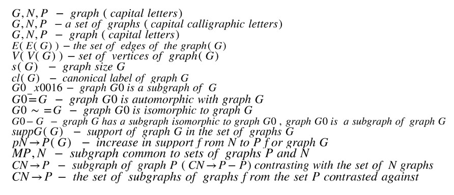
Directed Graph Theory: An overview of the basic concepts and properties of directed graphs and their application in cyber security. Modelling and Visualisation: Techniques for modelling and visualising data flows and relationships between systems using directed graphs. Graph Analysis Algorithms: Development and implementation of algorithms for analysing attack paths, detecting cycles and unusual patterns in graphs. Practical Cases: Analysis of real cases of cyber-attacks using directed graphs, identification of vulnerabilities and proposal of protection measures. Evaluation of Effectiveness: Evaluation of the effectiveness of the proposed methods and tools in real scenarios and their comparison with existing techniques. In the following, the symbolic designations of the formulas used in the paper, by which the individual graph models are described, are presented:

the set of graphs N ; the set of contrasting subgraphs characteristic of the set of graphs P with respect to the set of graphs N

The aim of this paper is to discuss and analyse the use of a pattern for the automatic classification of structures relating to graphs. The author of this paper proposed an algorithm using appropriate contrast patterns and common patterns. The algorithm was developed on the basis of a domain-wide method. The collected information was visualised on the basis of an appropriately selected algorithm for a given graph.

The paper is based on the thesis: “It is possible to develop a universal, modular, scalable, simple and, above all, efficient algorithm for object classification, modelled by graph structures, using minimal structural contrast patterns.”

The study was based on a statistical and descriptive summary of the algorithm created. It presented descriptive and methodological information. Its conclusions were related to the material as a whole.

The work is based graphs and solid graph

General Information on Graphs

A regular graph of degree n (n-regular graph) is a graph in which all vertices are of degree n.⁵

A full (complete) graph is a simple graph in which for every pair of vertices there is a connecting edge. A complete graph on vertices has card(E(G)) = n(n 2 -1) edges and is denoted by: Kn.⁶

A tree is a coherent acyclic graph (it has no cycle). Trees are used to represent hierarchies of data. In computer science, many data structures are based on a tree topology (e.g. binary trees, search trees, balanced AVL trees)⁷ The vertices of a graph represent specific data, while the edges represent relationships between them (e.g. parent-child relationships).⁸

Random graphs are another type of graphs affecting the present analysis.

A random (random) graph is one that is generated by a stochastic process. Many algorithms have been proposed to generate such graphs. They have a similar workflow, which involves randomly connecting an initial set of n vertices with edges. The most popular Erd˝os-Rényi model [Bol01]

(denoted by G(n, p)) assumes that edges are inserted independently between each pair of vertices with probability p. The expected value of the number of edges of a random graph is  .

Random graphs are often used in probabilistic processes aimed at proving the existence of a graph with certain predetermined properties.⁹

The following are basic typologies of graph structures that are often used to describe quantitative databases and the quality of databases.

By detecting relevant patterns relating to graph descriptions, appropriate criteria are determined, an example of which is support.  It represents a more computationally complex task than similar criteria described on the basis of numerical summaries. One of the most labour-intensive tasks is to produce solutions to subgraph isomorphism problems. The literature distinguishes two basic approaches to discovering graph patterns.¹⁰

The first is based solely on the detection of coherent subgraphs. The second, on the other hand, is complementary to the first and involves detecting all subgraphs as well as the inconsistent ones.

Using subgraphs increases the likelihood of obtaining an appropriate analysis.¹¹ Graphs are usually represented in a variety of ways, usually by a two-dimensional plane. It is based on the principle that vertices are connected by edges. They are usually represented on the basis of two basic parameters, namely, time complexity and memory complexity. Data are usually described on the basis of a neighbourhood matrix.¹²

The neighbourhood matrix stores information relating to the connections between vertices of graph G. This matrix is of dimension card(V (G)) on card(V (G)) and its columns and rows are indexed by the consecutive vertices of the graph. The element of matrix A contains the value of the edges starting from a given vertex. It can be used to record a given oriented and non-oriented graph. When referring to simple graphs, it refers to a specific set.¹³

The data structure defining the matrix above is based on very low time complexity. The basic operations performed on the matrix, i.e. deletion, addition, checking whether there are enough edges corresponding to the correct interval between edges, are performed in constant time. Operating quickly, there is a higher memory requirement O(card(G(V ) 2 )).¹⁴

When choosing an appropriately selected structure, it is first necessary to select the appropriate type of operation performed with the graphical representation of the data.  In practice, the matrices selected usually use graphs with a small number of vertices due to their high memory complexity. Given large graphs with a larger number of edges, it is necessary in this case to extract an appropriate amount of list-based data. The figure below shows a graphical representation of the data based on the matrices discussed above.

The table above shows a graphical representation of the relevant matrices on the basis of which the corresponding directed data analysis can be created on the basis of the selected graph. The data contained are numbered on the basis of specific Arabic numerals, while the edges are identified using Roman numerals.

Overview of Basic Methods and Problems

The fundamental problem associated with the hypothesis relating to the integral is the problem of isomorphism. This problem involves determining whether one graph is adequately contained in another. From a practical point of view, this can be determined by checking whether the principal graph contains an isomorphic subgraph contained in the base of the algorithm. Relative to the latter, the subgraph isomorphism problem is much more difficult and belongs to the class of NP-complete decision problems. The proof of NP-completeness is based on a reduction of a classical NP-complete problem: the problem of finding a clique in a graph [GJ90].¹⁵ Acting on the basis of the classical universal algorithm, one solves the algorithmic problem based on the method of complete review of all isomorphisms of a subgraph. Indeed, applying the subgraph isomorphism problem often takes a different form from the standard one. Typically, two types of graphs are used in this type of algorithm: a set of model graphs and a set of graphs. The difference between the two is that model graphs are taken into account when a reaction of an algorithm occurs.¹⁶ Then, when a problem arises, in order to solve it, one has to determine for the graph another set of subgraphs isomorphic to the model graph contained in the input graphs. Knowing the appropriate structure of the model graphs is used to analyse the designed algorithm in the preprocessing phase, referring to the acceleration of classification.

This paper is based on an algorithm, the purpose of which is to solve the subgraph isomorphism problem referring to the polynomial (O(n) = n 4 ) as a function of the total number of vertices in the model graphs. Preprocessing involves, among other things, transforming the sets of a given graph into a decision tree model in which the individual columns and rows of the matrix are stored. The problem, which is a huge disadvantage, is the huge internal memory requirement through the construction of the decision tree. In the extreme case, this demand increases as the total number of vertices in the model graph increases. This then limits the ability to make a sufficient number of solutions. The canonical label of the graph is worth mentioning at this point.¹⁷

The basis for presenting a suitable graph matrix is its representation, but it is not always mutually ambiguous. Its representation usually determines the topography being analysed without determining its representation. Every graph has a number of different representations; usually they are of the same type depending on how its edges and vertices are ordered. For example, any graph has (card(V (G)))! s neighbourhood matrix and (card(V (G)))! ∗ (card(E(G)))! of the neighbourhood incidence matrix and neighbourhood lists. The ambiguity of the algorithm means that, in most cases, it is not possible to quickly determine whether two representations are of the same graph. To answer the problem described above, a computationally expensive isomorphism needs to be created.¹⁸

The canonical label of a graph cl(G) is an unambiguous, deterministic representation of the graph in the form of a code (character string). Each graph has only one canonical label. It is independent of the ordering of vertices and edges, and is fully determined by the topology of the graph (and any labels of vertices and edges). Furthermore, the canonical label determines the topology of the graph, i.e. knowledge of the label is synonymous with knowledge of the graph structure.¹⁹ The basic properties of the canonical label of a graph follow from its definition. Usually such algorithms include labels; a label which determines the isomorphism of graphs (i.e. isomorphic graphs have the same label: G0 ∼= G ⇐⇒ cl(G0 ) = cl(G))) and labels that define an ordering relation between the graphs (i.e. G0 < G ⇐⇒ cl(G0 ) < cl(G)).²⁰

The definition of a label does not specify either its method or its content. A common approach is to arrange the rows, columns and notation appropriately by referring to the relevant character string. Determining the appropriate label then boils down to finding a code that is their minimal graphical lexicon. Thus, by looking for vertices to which a minimal matrix corresponds, the corresponding vertices are determined (card(V (G))!).²¹

Canonical labels are mainly used to solve the isomorphism problem. The computational cost of determining the canonical labels of a graph is comparable to the cost of a single isomorphism test between two graphs of the same size.

On the other hand, the time cost associated with comparing two canonical labels (i.e. isomorphism statements) is negligible compared to the former. The use of canonical labels is, therefore, particularly desirable where individual graphs participate in isomorphism tests repeatedly.²²

The canonical label can also be used as an alternative method. Its undoubted advantages include: one-dimensionally small memory requirements (mapping cl(G) → G as well as G → cl(G)), determinism, no restrictions on the structure of the represented graph and well-defined and order.

The result of these advantages is used as an index in graph databases. The property of order relations guarantees the execution of search operations in logarithmic time (binary search). On the other hand, it has a number of disadvantages: it is intended to be read-only, almost none of the operations typical of other graph representation methods can be dug out, and it is not very human, readable and understandable.²³

The practical application of canonical labels can testify to the fact that comprehensive, impressive hardware solutions are available to support their calculation process. The proposed hardware architecture runs 10 to 100 times faster than a software solution.

An important aspect of the article is the determination of the support coefficients responsible for qualitatively defining the given algorithm. The next subsection describes the support of a given algorithm.

Analysis of the Graph Algorithm based on the Contrast Common Pattern Classifier (CCPC) Method

This subsection discusses the CCPC concept on the basis of which the attack graph algorithm was created. It is based on the contrast pattern, on which the basic properties were created and its operation is discussed. The primary task of the method is to classify data depicted on the basis of graphs. However, in this type of method, it is not always possible to use the appropriate subgraphs in order to obtain a suitable algorithm. If classification is still not possible, then the graph will remain unclassified. The operation of the algorithm results in the determination of membership coefficients for the corresponding test graph taking into account the individual decision classes. The membership coefficients are calculated using the relevant support parameters and the increase in support of the test graph’s subgraphs, which are contrastive or common subgraphs. Determining the appropriate coefficients is based on the design of the corresponding schema using a relational database.²⁴

Suppose that G is a set of training graphs and T is a text graph. The master graphs given the algorithm are divided into subsets of graphs belonging to the same decision group as defined by the algorithm: G1, …, Gn; G = S i=1..n Gi . Let C( Min GGi)→Gi be the set of all minimal contrastive subgraphs for Gi relative to the set of graphs (G Gi), where i ∈ h1, ni . Let MMin G1,…,Gn be the set of all minimal common subgraphs for G1, …,Gn .²⁵

The proposed classification algorithm requires the selection of ways to calculate the coefficients of decision class membership. A strategy for calculating the coefficient based on contrasting (i.e. scConA or scConB) and common (i.e. scComA or scComB) subgraphs is needed.²⁶

The general scheme of the CCPC algorithm is based on the following steps:

1. Determine the value of the scConA(T) (scConB(T)) coefficients for all decision classes.
2. Assign the test graph T a class label that corresponds to the largest value of scConA(T) (scConB(T)).

If classification is not possible then:

(a) Determine the value of the coefficients scComA(T) (scComB(T)) for those decision classes for which the value of the coefficient scConX is maximum (i.e. scConX(T) = max(scConX(T))).

(b) Assign to the test graph T the class label that corresponds to the largest value of scComA(T) (scComB(T)). If classification is not possible then leave the graph as unclassified.²⁷

Based on the assumptions discussed above, an algorithm based on the attack cycle in relation to the attack graph was constructed. The following table presents an example database with training graphs (Z). The graphs were divided into two disjoint subsets according to the decision class membership (Z = ZA S ZB).

The choice of the above representation base for certain algorithms is conditioned on the criteria: runtime and memory requirements. Taking into account the above classification, all subgraphs are represented in a way that makes it possible to examine the corresponding graph pattern reflecting the database and the algorithm contained in it. When performing this type of operation, time is critical to the quality of the algorithm. Graphs are usually represented on the basis of structures, occupying little memory. Given these specific conditions and limitations, the best way to represent the detected subgraphs will be the canonical label.²⁸

The canonical label does not impose any additional restrictions on the graph topology (e.g. graph orientation) and labels. Knowledge of specific properties is usually used to design an appropriate canonical label.²⁹

Characterisation of the Attack Cycle based on a Selected Graph Algorithm

Given the analysis of cyber-attack cases to date, it is worth noting in them a certain systematic repetition of a given pattern, which the literature refers to as the process of a cyber-attack. The literature perceives this attack as a short-lived event that cannot be countered. Indeed, it is a momentary process, for which a specific set of actions performed in the right order with respect to time and place of duration is gathered.³⁰

This work considers the general life cycle of attacks in relation to the following phases:     

• (S1) identification and definition of attack targets – pre-planning,
• (S2) reconnaissance,
• (S3) weaponisation,
• (S4) delivery of malicious code,
• (S5) launch and control of malicious code (cyber execution and command & control),
• (S6) achievement of objectives,
• (S7 ) end of attack and cover-up of tracks.³¹

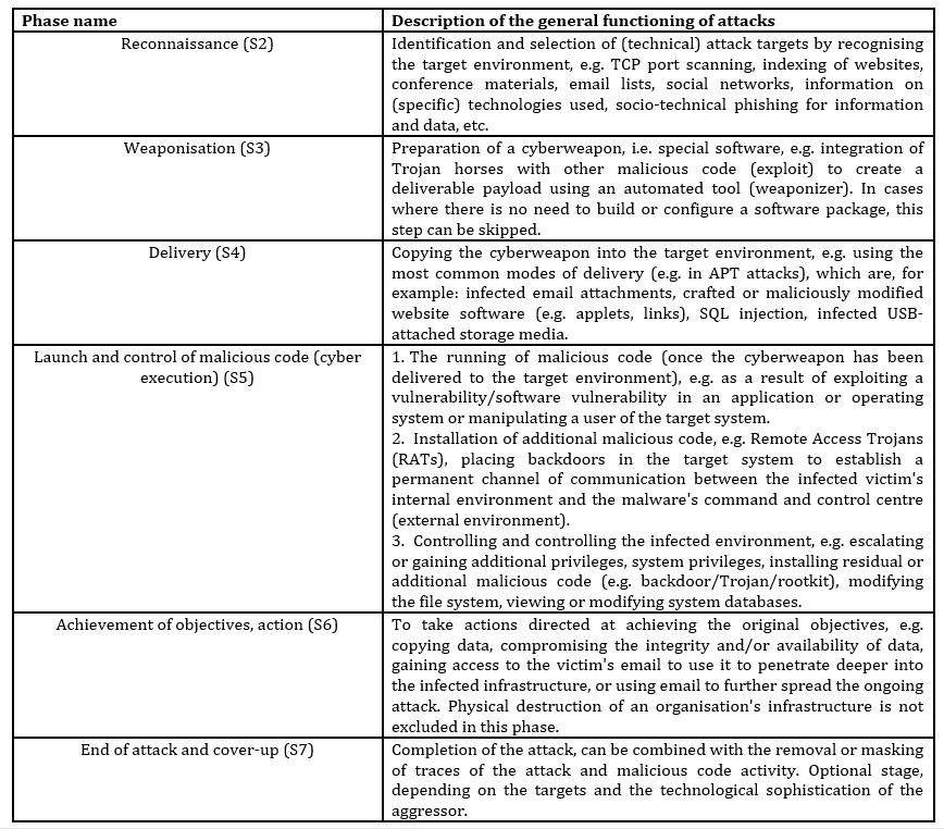
The literature considers two basic cycles of attack activity, namely: S1 and S3. The aforementioned phases refer, practically speaking, to the planning and termination of attacks. The other cycles of attack algorithms are reflected in the literature and are described based on the table below.

Table l: Phases of the overall life cycle of a cyber-attack

^{Source: I. H. Witten and E. Frank. Data Mining: Practical Machine Learning Tools and Techniques, Second Edition (Morgan Kaufmann Series in Data Management Systems). Morgan Kaufmann Publishers Inc., San Francisco, CA, USA, 2005.}

This table illustrates an analysis of the general emergence of the life cycle of a cyber-attack. Creating a picture of it on the basis of the graph, it is noted that there is no possibility of returning, given time and space, to its initial phases and that each of them must occur one after the other. Each of the phases has its own dynamics of the attack process.The figure below allows us to illustrate in graphical form how the transitions between the different phases of an attack are directed.

From a practical point of view, an attack on an organisation or a company, an institution usually has no end in sight. This type of attack, given its systematic manner, pretends to have an effect without assuming that time is an important factor in the process. Once the intended effect is achieved, a new target is set, starting all over again. It is, therefore, assumed that cyber-attacks can be repeated and that the interruption of the current attack results in the attacker starting a new cycle.³²

Based on the diagram above, referring to the method described above, the present algorithm was built.

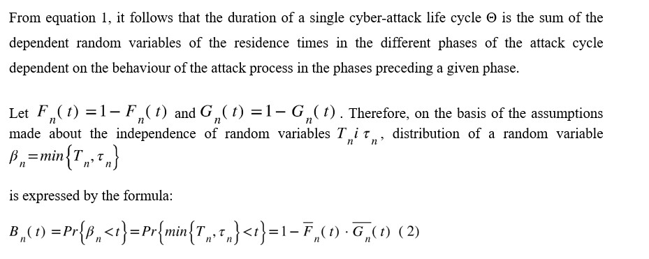
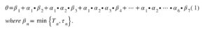
Let us assume that Tn ∈ [0, +∞)) denotes the time necessary to successfully complete the Sn phase (n = 1, 2, …, 7). Hereafter, we will refer to these times as the necessary phase durations. We assume that Tn is a random variable with distribution Fn (t) = Pr{Tn< t} and finite expectation value ETn (ETn = ∫0 +∞tdFn (t) < +∞). Let τn ∈ [0, +∞) be a random variable with distribution Gn (t) = Pr{τn< t} and finite expectation value Eτn (Eτn = ∫0 +∞tdGn (t) < +∞) denoting the time after which a stop can occur. Here, for the sake of generalisation, we will make the assumption that the current attack cycle can also end in the pre-planning phase. Therefore, the dwell time in each Sn phase is equal to βn = min{Tn , τn} (n = 1, 2, …, 7). A conforming graph of transitions between states is shown in Figure 2. The return to state S1 symbolises the start of a new cyber-attack – a new cyber-attack cycle. The arcs of the graph of transitions between phases of the cyber-attack cycle are described by the times that may be followed by a transition to the next phase or, as a last resort, the termination or interruption of the attack.³³

Here, it is additionally assumed that the necessary durations of the individual phases are stochastically independent, i.e. the random variables T1 , …, T7 are independent random variables. Furthermore, let the random variables τ1 , …, τ7 also be independent random variables. Stochastic independence of the random variables Tn and τn (n = 1, 2, …, 7) is also assumed.

Duration of a Single Cyber-attack Cycle

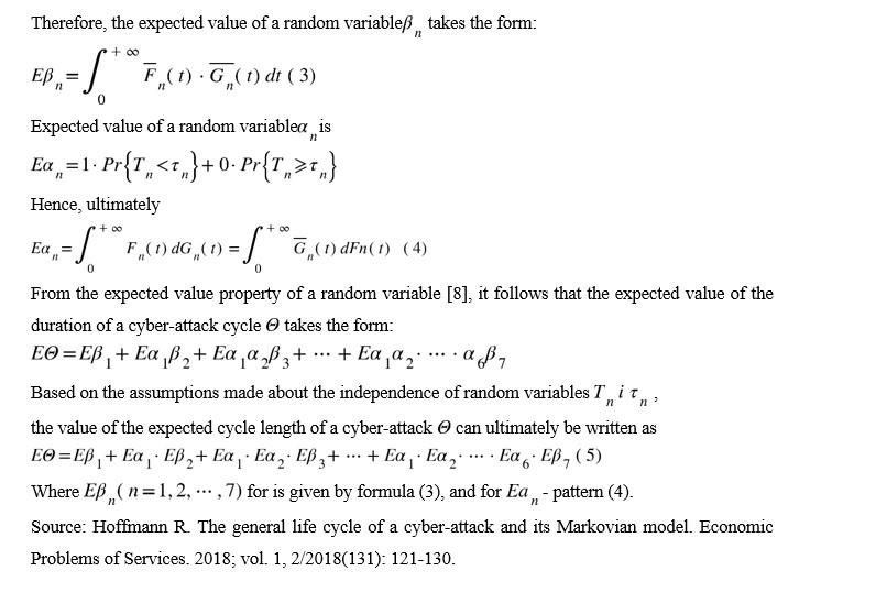
Assume that αn ∈ {0,1} for each n = 1, 2, … 7 is a binary random variable** – such that αn = 1 when the event {Tn < τn} occurs and αn = 0 when {Tn ≥ τn} occurs. Let Θ ∈ [0, +∞) denote the duration of a single cyber-attack cycle. Given the designations and assumptions made, the duration of a single cyber-attack cycle Θ can be written as follows:

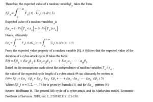
Source: Hoffmann R. The general life cycle of a cyber-attack and its Markovian model. Economic Problems of Services. 2018; vol. 1, 2/2018(131): 121-130.

The above-described algorithms illustrate a model of the general life cycle of attacks based on a graph drawn up accordingly. Based on the literature, this cycle moves on the basis of two phases: identification and definition of targets, which are considered as planning. Given that, the chosen graph model is based on a layout drawn up on the principle of a graph defining the different phases of its cycle. It is assumed that the attack can be aborted while the aggressor is in any phase of the attack. In practice, the interruption of the attack can occur not only at the will of the cybercriminal, but also, and perhaps above all, because of the cyber defence system in operation.³⁴

Taking into account the developed graph model, a data analysis based on the stationary probability of the individual phases of its action was calculated, which found the individual action relating to its practical application.  It should be pointed out here that, from a practical point of view, it is necessary and sufficient to know the expected values of the individual times and to estimate the probability of success of the completion of the individual phases of the attack cycle in order to estimate the above characteristics.³⁵

The easiest to classify turned out to be set number 1, which was so that the set was the smallest. All algorithms (except random and frequency) achieved a classification accuracy of. The graph model proved superior to the hybrid model. The algorithm based on determining the maximum common subgraph achieved near classification efficiency for a graph of size 30 vertices. The CCPC algorithm needed 20 more vertices to get a better result.

For set number 2, algorithms using the hybrid representation achieved the highest classification accuracy. The CCPC algorithm was superior to the other methods based on the graph model. Set number 3 was the largest set available. In this case, the CCPC algorithm was the best algorithm. The same classification accuracy was achieved by a method with clever feature extraction of subgraphs based on the hybrid model, but it needed three times as many features (120 features) as the CCPC algorithm (40 features). For the last collection of K7-series documents, the CCPC algorithm again achieved the best classification accuracy.³⁶

In summary, the CCPC algorithm proved to be the best algorithm for three of the four datasets analysed. For collection number 4, it scored worse than the leader in this category. The algorithm using the hybrid document representation had a better classification performance in this case.

Experimental studies conducted on four real-world datasets confirm the height of the effectiveness of the method based on contrast patterns for document classification.

The CCPC algorithm achieved the best accuracy among the methods analysed, for three collections of websites. The proposed algorithm makes it possible to assign a category to a web page describing its subject matter without necessity. It can be used in search engines as well as in knowledge portals to replace the manual categorisation of documents with an automatic process and to provide higher as a service.

Conclusions

 On the basis of the above-discussed analysis of the database relating to four real-world sets, which confirm the height, and at the same time the effectiveness, of a method based on contrasting patterns developing the relevant phases of attack cycles, the CCPC algorithm best classifies the attack data among the other methods building the database.

The proposed algorithm makes it possible to read graphically depicted data. Algorithms are used to describe subjects without the need for human resources. This type of database is usually used via a web search and also on a knowledge basis to replace paper documentation using an automatic process to provide the individual phase of attack cycles, which translates into the quality and speed of the detected information.

Notes

[1]A. Voznica, A. Kalousis, and M. Hilario. Kernels over relational algebra structures. In T. B. Ho, D. W. L. Cheung, and H. Liu, editors, PAKDD, volume 3518 of Lecture Notes in Computer Science, pages 588-598. Springer, 2005.

² J. R. Ullmann. An algorithm for subgraph isomorphism. J. ACM, 23(1):31-42, 1976.

3 R. Albert, H. Jeong, and A. L. Barabási. The diameter of the world wide web. Nature, 401:130, September 1999.

⁴A.L. Barabási, H. Jeong, Z. Neda, E. Ravasz, A. Schubert, and T. Vicsek. Evolution of the social network of scientific collaborations. Physica A, 311:3, 2002.

⁵ J. Bailey and G. Dong. Contrast Data Mining: Methods and Applications., 2007. tutorial presented at the IEEE International Conference on Data Mining (ICDM).

6 R. Albert and A. L. Barabási. Statistical mechanics of complex networks. Review of Modern Physics, January 2002.

7 Pawel Gawrychowski, Haim Kaplan, Shay Mozes, Micha Sharir, and Oren Weimann. Voronoi diagrams on planar graphs, and computing the diameter in deterministic O˜ (n 5/3) time. In Proceedings of the Twenty-Ninth Annual ACM-SIAM Symposium on Discrete Algorithms, SODA 2018, New Orleans, LA, USA, January 7-10, 2018, pages 495-514, 2018.

8Andrew V. Goldberg. Scaling algorithms for the shortest paths problem. SIAM J. Comput., 24(3):494-504, 1995.

⁹ Philip N. Klein and Shay Mozes. Optimization algorithms for planar graphs, 2017.

¹⁰ D. J. Cook and L. B. Holder. Mining Graph Data. Wiley, 2006.

¹¹A. Dominik and J. Wojciechowski. Analysis of the structure of online marketplace graph. In M. A. Klopotek, S. T. Wierzchon, and K. Trojanowski, editors, Intelligent Information Systems, Advances in Soft Computing, pages 243-252. Springer, 2006.

¹²Z. Harchaoui and F. Bach. Image classification with segmentation graph kernels. In CVPR. IEEE Computer Society, 2007.

¹³L. B. Holder, D. J. Cook, and S. Djoko. Substructure discovery in the subdue system. In Proceedings of the Workshop on Knowledge Discovery in Databases, pages 169-180, 1994.

¹⁴Ibid.

¹⁵P. Faliszewski. The structure of the class np. Master’s thesis, AGH University of Science and Technology, 2004.

¹⁶J. Łącki and P. Sankowski. Optimal decremental connectivity in planar graphs. Theory Comput. Syst., 61(4):1037-1053, 2017

¹⁷G. Dong, X. Zhang, L. Wong, and J. Li. CAEP: Classification by aggregating emerging patterns. In Discovery Science, pages 30-42, 1999.

¹⁸G. Dong, X. Zhang, L. Wong, and J. Li. CAEP: Classification by aggregating emerging patterns. In Discovery Science, pages 30-42, 1999.

¹⁹T. H. Grubesic, M. E. O’Kelly, and A. T. Murray. A geographic perspective on commercial internet survivability. Telematics and Informatics, 20(1):51-69, 2003.

²⁰J. Huan, W. Wang, and J. Prins. Efficient mining of frequent subgraphs in the presence of isomorphism. In ICDM, pages 549-552. IEEE Computer Society, 2003.

²¹T. Kudo, E. Maeda, and Y. Matsumoto. An application of boosting to graph classification. In NIPS, 2004.

²²G. S. Lueker and K. S. Booth. A linear time algorithm for deciding interval graph isomorphism. J. ACM, 26(2):183-195, 1979.

²³T. M. Mitchell. Machine Learning. McGraw-Hill Higher Education, 1997.

²⁴F. Sadikoglu, S.Uzelatinbulat, Biometric retina identification based on neural network. Procedia Computer Science. 2016; 102: 26-33.

²⁵M. J. Zaki. Scalable algorithms for association mining. IEEE Transactions on Knowledge and Data Engineering, 12(3):372-390, 2000.

²⁶Z. Zeng, J. Wang, and L. Zhou. Efficient mining of minimal distinguishing subgraph patterns from graph databases. In T. Washio, E. Suzuki, K. M. Ting, and A. Inokuchi, editors, PAKDD, volume 5012 of Lecture Notes in Computer Science, pages 1062-1068. Springer, 2008. 120

²⁷Ibid.

²⁸J. R. Ullmann. An algorithm for subgraph isomorphism. J. ACM, 23(1):31-42, 1976.

²⁹C. Joost van Rijsbergen. Information Retrieval. Butterworths, London, 2nd edition, 1979.

³⁰David Weininger. Smiles, a chemical language and information system. 1. introduction to methodology and encoding rules. Journal of Chemical Information and Computer Sciences, 28(1):31-36, 1988.

³¹Ibid.

³²C. Joost van Rijsbergen. Information Retrieval. Butterworths, London, 2^nd edition, 1979.

³³L. Babai and E. M. Luks. Canonical labeling of graphs. In STOC ’83: Proceedings of the 15th Annual ACM Symposium on Theory of Computing, pages 171-183, New York, NY, USA, 1983. ACM

³⁴R. Hoffmann, The general life cycle of a cyber-attack and its Markovian model. Economic Problems of Services. 2018; vol. 1, 2/2018(131): 121-130.

³⁵ GP.Klimow,Processes of mass service. Warsaw: WNT; 1979.

³⁶Ibid.

Bibliography

• Albert and A. L. Barabási. Statistical mechanics of complex networks. Review of Modern Physics, January 2002.
• Aery. Infosift: Adapting graph mining techniques for document classification. Master’s thesis, The University of Texas at Arlington, December 2004.
• V. Aho and J. E. Hopcroft. The Design and Analysis of Computer Algorithms.
• Addison-Wesley Longman Publishing Co., Inc., Boston, MA, USA, 1974.
• Albert, H. Jeong, and A. L. Barabási. The diameter of the world wide web. Nature, 401:130, September 1999.
• Agrawal and R. Srikant. Fast algorithms for mining association rules. Readings in database systems (3rd ed.), pages 580-592, 1998.
• Borgelt and M. R. Berthold. Mining molecular fragments: Finding relevant substructures of molecules. In Proceedings of the 2nd IEEE International Conference on Data Mining, pages 51-58, Washington, DC, USA, 2002. IEEE Computer Society.
• L. Barabási and E. Bonabeau. Scale-free networks. Scientific American,pages 50-59, May 2003.
• Bailey and G. Dong. Contrast Data Mining: Methods and Applications., 2007. tutorial presented at the IEEE International Conference on Data Mining (ICDM).
• Babai, D. Y. Grigoryev, and D. M. Mount. Isomorphism of graphs with bounded eigenvalue multiplicity. In STOC ’82: Proceedings of the 14th Annual ACM Symposium on Theory of Computing, pages 310-324, New York, NY, USA, 1982. ACM.
• L. Barabási, H. Jeong, Z. Neda, E. Ravasz, A. Schubert, and T. Vicsek. Evolution of the social network of scientific collaborations. Physica A, 311:3,2002.
• M. Borgwardt and H. P. Kriegel. Shortest-path kernels on graphs. IEEE International Conference on Data Mining, 0:74-81, 2005.
• Babai and E. M. Luks. Canonical labeling of graphs. In STOC ’83: Proceedings of the 15th Annual ACM Symposium on Theory of Computing, pages 171-183, New York, NY, USA, 1983. ACM.
• J. A. Berry and G. S. Linoff. Data Mining Techniques: For Marketing, Sales, and Customer Relationship Management. John Wiley & Sons, 2004.
• L. Barabási and Z. N. Oltvai. Network biology: Understanding the cell’s functional organization. Nature, 5:101-113, February 2004.
• L. Bodlaender. Polynomial algorithms for graph isomorphism and chromatic index on partial k-trees. In No. 318 on SWAT 88: 1st Scandinavian Workshop on Algorithm Theory, pages 223-232, London, UK, 1988. Springer-Verlag.
• Bollobas. Random Graphs. Cambridge University Press, 2001.
• A. Bondy. Graph Theory with Applications. Elsevier Science Ltd, 1976.
• Bunke and K. Shearer. A graph distance metric based on the maximal common subgraph. Pattern Recognition Letters, 19(3-4):255-259, 1998.
• Chakrabarti and C. Faloutsos. Graph mining: laws, generators, and algorithms. ACM Computing Surveys, 38(1), March 2006.
• J. Cook and L. B. Holder. Mining Graph Data. Wiley, 2006.
• Crucitti, V. Latora, M. Marchiori, and A. Rapisarda. Efficiency of scale-free networks: Error and attack tolerance. Physica A, 320:642, 2003.
• J. Colbourn. On testing isomorphism of permutation graphs. Networks, 11:13-21, 1981.
• Chen, X. Yan, P. Yu, J. Han, D. Zhang, and X. Gu. Towards graph containment search and indexing. In Proceedings of the 33rd International Conference on Very Large Data Bases, VLDB 2007, pages 926-937. VLDB.
• K. Debnath, R. L. Lopez de Compadre, G. Debnath, A. J. Shusterman, and C. Hansch. Structure-activity relationship of mutagenic aromatic and heteroaromatic nitro compounds. correlation with molecular orbital energies and hydrophobicity. Journal of Medicinal Chemistry, 34:786-797, 1991.
• Daszczuk, P. Gawrysiak, T. Gerszberg, M. Kryszkiewicz, J. Miescicki, M. Muraszkiewicz, M. Okoniewski, H. Rybiński, T. Traczyk, and Z. Walczak. Data mining fortechnical operation of telecommunications companies: a case study. 2000. 4th World Multiconference on Systemics, Cybernetics and Informatics (SCI’2000).
• Diestel. Graph Theory. Springer-Verlag, New York, USA, 2000.
• Deshpande, M. Kuramochi, and G. Karypis. Frequent sub-structure-based approaches for classifying chemical compounds. In Proceedings of the 3rd IEEE International Con- 110
• Dong and J. Li. Efficient mining of emerging patterns: Discovering trends and differences. In KDD ’99: Proceedings of the fifth ACM SIGKDD International Conference on Knowledge Discovery and Data Mining, pages 43-52, New York, NY, USA, 1999. ACM Press.
• Dominik. Data analysis using rough set theory. Master’s thesis, Warsaw University of Technology, 2004.