Anisotropic Graph Search on Multi-Layer Terrain Maps for Mobile Robot Path Planning

Introduction

Autonomous navigation in unstructured terrain is one of the most complex tasks in mobile robotics. Graph-search planners perform reliably in indoor and structured environments, but their use off-road and on uneven ground is restricted by a fundamental limitation: a path that is shortest in the geometric sense need not be the most suitable one for the vehicle. On rough terrain, the quality of a path is determined not only by its length and its clearance from obstacles, but also by elevation changes, the orientation of local slopes, surface properties, and the heading of the robot with respect to the terrain geometry. Consequently, a geometrically short path may require excessive energy, impose unfavorable dynamic loads, or pose danger to the vehicle itself.

Modern path planning algorithms originate from shortest-path search on weighted graphs. Dijkstra’s algorithm provided the established framework for optimal search when edge costs are nonnegative (Dijkstra, 1959; Waga et al., 2025; Tang et al., 2025). A* introduced heuristic guidance into this framework, which considerably decreases the number of node expansions and, under standard assumptions, does not compromise optimality (Hart et al., 1968; Pohl, 1970; Waga et al., 2025; Xuan et al., 2025). Further developments adopted several different approaches. Incremental replanning methods, e.g., D* and D* Lite, address changing or partially known maps and limit computation by reusing the results of previous searches (Stentz, 1994; Koenig and Likhachev, 2002; Waga et al., 2025; AbuJabal et al., 2024). Anytime algorithms, e.g., ARA* and AD*, first provide a solution of bounded suboptimality and then improve it iteratively, which is beneficial for robots operating in real time (Likhachev et al., 2003; Likhachev et al., 2005; Xuan et al., 2025). Geometry-aware approaches, e.g., Field D* and Theta*, mitigate the artifacts of motion restricted to grid edges and in many cases produce shorter or smoother trajectories (Ferguson and Stentz, 2006; Nash et al., 2007; Waga et al., 2025; Tang et al., 2025).

Most graph-search methods treat traversal costs as isotropic – such approach is acceptable in structured environments. On rough terrain, however, it is an oversimplification, because an ascent differs from a descent, and lateral traversal of a slope can be considerably more dangerous than motion along its gradient. The cost of a given local transition therefore depends on the direction of travel, causing the planning problem to become anisotropic. This property is especially important for robots working in complex, unstructured environments like forests, quarries or dunes, where the quality of a path depends on robot safety as much as it does on optimality.

Such difficulties gave rise to a considerable number of studies on traversability assessment and terrain-aware planning. According to recent surveys (Beycimen et al., 2023; Benrabah et al., 2024; Carvalho et al., 2025), the navigation of unmanned ground vehicles is increasingly based on layered environment representations that combine geometry and models of vehicle–terrain interaction. Traversability is commonly estimated on the basis of digital elevation models, point clouds, or sensor data and is passed to the planner as a costmap. Within this framework, Wang et al. (2024) and Liu et al. (2024) proposed an improved A*-based planner for uneven terrain, in which models of trafficability and ruggedness obtained from elevation data are combined. Their results confirm that planning reliability increases when the local terrain geometry is represented explicitly in the cost function, rather than being reduced to a binary distinction between obstacles and free space. A separate group of studies concerns deformable or mixed terrain, on which mobility is constrained by slip and traction as well as by geometry. Sakayori and Ishigami (2024) and Nishishita and Ishigami (2025), for instance, included slip-rate-dependent traversability in the path costs of wheeled robots on sand and showed that the explicit representation of terrain-dependent motion effects may improve path quality considerably.

The presented study focuses on anisotropic cost models for terrain navigation. These models express the traversal cost as a function of the robot heading with respect to the slope, distinguishing between ascending, descending, and lateral motion on inclined ground. A continuous formulation of anisotropic costs for irregular terrain was introduced by Sánchez-Ibáñez et al. (2023), and the growing role of terrain-aware traversability modeling in unstructured environments was pointed out by Carvalho et al. (2025). Both works show that anisotropy has a physical basis in the mechanics of terrain traversal. In most existing studies anisotropic planning is formulated within continuous optimal control and combined with planners other than graph search, even though graph-based methods are widely used in robotics, as they are simple, predictable, and relatively cheap in computing power needed. The method described in this paper therefore preserves the classical A* scheme and supplements it with an anisotropic, terrain-dependent transition model. This model can be embedded in a standard grid-based planner and evaluated against simpler variants in the same software environment. The resulting planner, referred to as Terrain-Aware Anisotropic A* (T-AAA*), uses three co-registered map layers: an inflated obstacle map, an elevation map, and a terrain-multiplier map. Its edge cost combines the 3D geometric distance, penalties related to the surface, a signed pitch factor, and a roll factor that depends on the heading; both slope-related factors are obtained from the local height gradient. In the resulting directed weighted graph, the cost of a transition depends on the pair of adjacent cells and, additionally, on the direction in which the terrain is traversed. The planner is thus able to select longer routes when they are safer to traverse.

The paper makes two contributions. The first is a formal description of T-AAA*. The second is an experimental comparison between the complete method and four variants obtained by its systematic simplification, namely Dijkstra, A*, A* with terrain multipliers, and A* with pitch/roll penalties. Such a comparison allows the effect of each cost layer to be identified separately and indicates the terrain conditions in which the full anisotropic formulation offers an advantage. Six benchmark datasets were used, covering flat, urban-like, off-road, dune-like, and mountain-pass terrain.

The paper is organized into four sections. Following this introduction, Section 2 presents the Terrain-Aware Anisotropic A* method together with the map representation, the cost functions dependent on direction, and the variants used in the benchmark. The experimental setup and the results obtained for the six benchmark datasets are reported in Section 3. Section 4 discusses the results and indicates possible directions of further research.

Terrain-Aware Anisotropic A*

Map Representation

The planner uses three map representation layers:

• Obstacle map Board ∈ R^H×W, where free cells contain 0 and occupied cells contain 1.
• Elevation map HeightMap ∈ R^H×W, storing the terrain heights from which 3D distances, pitch and roll angles, and slopes are computed.
• Terrain multiplier map TerrainMult ∈ R^H×W, containing per-cell cost multipliers that encode the relative difficulty of the terrain.

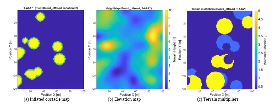
As a preprocessing step, the obstacles in the occupancy grid are inflated by r so that the footprint of the robot is taken into account. Figure 1 presents the three input layers of the benchmark: the inflated obstacle map, the elevation map, and the terrain-multiplier map.

Figure 1: Input layers of a representative benchmark map

Terrain multiplier map

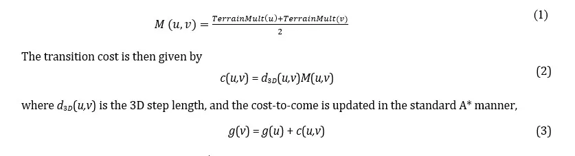
The planner uses a terrain multiplier map TerrainMult ∈ R^H×W. The scalar stored in each cell expresses the relative effort of crossing the local terrain, and this layer is incorporated directly into the transition cost used by A*.

For a directed move u → v, the terrain multiplier term is defined as the mean of the values at its two end cells,

Elevation-based geometric quantities

Each free cell in Board defines a graph vertex connected to its eight neighbors (8-neighborhood). For a node u = (r_u,c_u) and its successor v = (r_v,c_v), the horizontal displacement is given by

The elevation map HeightMap supplies the vertical component of motion, and the signed elevation difference between two adjacent cells is

where s_h is the vertical scale factor, equal to 1 in this study.

Combining both components gives the 3D step length:

Slope descriptors related to pitch and roll

For a move from u to v, two direction-dependent slope descriptors are derived from the elevation map. The pitch-related angle is determined by the elevation change along the direction of travel:

where positive values indicate ascent and negative values descent. The roll-related angle is based on the component of the local height gradient that is orthogonal to the travel direction:

where  denotes the in-plane unit vector perpendicular to the direction of motion from u to v.

Both penalty factors increase linearly with the corresponding angle, and an additional penalty multiplier is applied once the angle exceeds a prescribed threshold. For the pitch-related term,

where k_p is the pitch gain, θ_max is the pitch threshold, and λ_p > 1 is the additional penalty multiplier applied above this threshold.

For the roll-related term,

where k_r is the roll gain, ϕ_max is the roll threshold, and λ_r > 1 is the additional penalty multiplier applied above this threshold.

Full T-AAA* edge cost

The full T-AAA* planner combines the geometric, terrain, and directional slope terms into a single transition cost:

where d_3D(u,v) is the 3D step length, F_pitch(θ(u,v)) and F_roll(ϕ(u,v)) are the pitch- and roll-related penalty factors, and M(u,v) is the terrain multiplier term defined in Eq. (1). The simplified planner variants used for comparison are obtained by selectively removing individual terms:

Node ordering is the only aspect in which Dijkstra and the baseline A* differ: the local transition cost is the same, and a heuristic is used only by A*.

T-AAA* search procedure

Node selection in T-AAA* is identical to that in classical A*; the two algorithms differ only in the cost function. For each admissible move u → v, T-AAA* computes the 3D step length, the terrain multiplier term, and the pitch- and roll-related penalty factors, and combines them into the transition cost c_TA(u,v). The cost-to-come is then updated as:

while node ordering is based on:

where h(v) denotes the heuristic estimate of the remaining distance to the goal. In the baseline A* variant, h(v) is given by the Euclidean distance to the goal multiplied by the smallest terrain modifier, whereas Dijkstra is obtained by setting h(v) = 0. All remaining variants share this search procedure and differ only in the transition-cost function. The complete procedure is summarized in Algorithm 1.

Benchmark Setup and Results

Experimental protocol

The computations were performed in MATLAB, using a workstation with an Intel Core i9-13900KF processor and 32 GB of RAM.

The following five planners were compared:

1. Dijkstra,
2. A*,
3. A* + terrain multiplier,
4. A* + pitch/roll penalties,
5. T-AAA*.

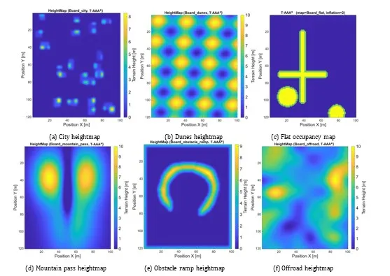
Each planner was tested on the same six benchmark datasets: Board_city, Board_dunes, Board_flat, Board_mountain_pass, Board_obstacle_ramp, and Board_offroad. Their height maps are shown in Fig. 2. For Board_flat, the occupancy grid is shown instead, because its height map contains no meaningful elevation data.

Figure 2: Benchmark maps used in the experiments

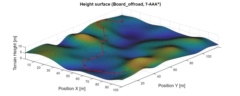
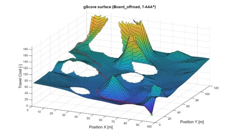
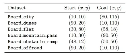
Because planner variants minimize different objectives, their native costs are not directly comparable. Therefore, each path was additionally evaluated with the full T-AAA* objective defined in Eq. (11), and, unless stated otherwise, the quantitative comparisons below refer to this terrain-aware re-evaluation. The start and goal points used by all algorithms are listed in Table 1, and Figures 3 and 4 show examples of the height surface and of the g-score (cost-to-come) surface.

Figure 3: Path on the 3D height surface of Board_offroad

Figure 4: Cost-to-come (g-score) surface of Board_offroad in 3D

Table 1: Start and goal positions for each benchmark dataset

Quantitative comparison

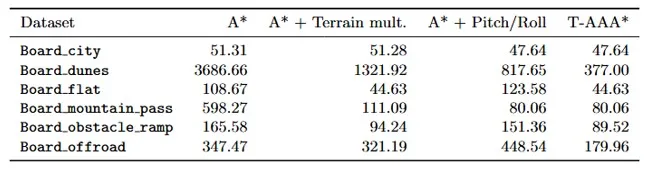
On Board_mountain_pass, restrictive terrain geometry limits feasible routes, making direction-dependent slope effects the dominant factor in path selection. Both the pitch/roll-aware and full T-AAA* planners therefore achieve identical best shared costs (Table 2).

Table 2: Shared T-AAA* path cost obtained by each method on every benchmark dataset

The differences between the methods are largest on the two most challenging terrains, Board_dunes and Board_offroad. On Board_dunes, the pitch and roll terms have a greater effect than the terrain multiplier. Where elevation differences are large, as in Board_mountain_pass, the terrain multiplier has smaller impact, and A* + Pitch/Roll attains the same cost as T-AAA*.

On Board_flat, T-AAA* and A* with the terrain multiplier attain the same best cost; because the terrain is level, the pitch and roll terms have no significant effect.

The advantage of combining both effects is most evident on Board_offroad. Neither the variant based only on surface information nor the variant based only on slope reaches the lowest cost, whereas T-AAA* reduces the shared cost to 179.96, compared with 321.19 for the terrain-multiplier variant and 448.54 for the pitch/roll variant.

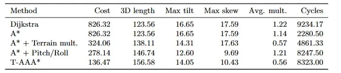
Table 3: Mean benchmark results over all six datasets, re-evaluated

under the shared T-AAA* cost model

Table 3 leads to three conclusions. First, a considerable difference is observed in search effort. A*, as the baseline for the cycles needed have a mean value of 2280.50. Each terrain-aware modification of cost function caused this values to increase: +113,2% (2280.50 vs 4861.33) for Terrain multiplier, +261,7% (2280.50 vs 8247.5) for Pitch/Roll and +264,9% (2280.50 vs 8323.0) for full T-AAA* cost calculation. What is noteworthy, combining both multipliers didn’t cause computational effort to increase meaningfully (8247.5 vs 8323.0), while cost decreased significantly: 278.14 vs 136.47.

Second, extending the A* cost function with only one group of terrain-related terms, i.e., either the terrain multiplier or the pitch and roll terms, already reduces the mean shared cost substantially. Compared with the baseline A*, the terrain multiplier reduces cost from 826.32 to 324.06, and the pitch and roll terms reduce it to 278.14. These results show that terrain model and elevation-based anisotropy both have high impact on path quality, but through different mechanisms. The terrain multiplier directs paths toward more favorable surfaces, whereas the pitch and roll terms penalize geometrically unfavorable motion, such as cross-slope traversal or steep ascents.

Third, the complete T-AAA* formulation achieves the lowest mean shared cost, 136.47, which is 83.5% lower than that of the baseline A*. The reduction remains substantial in comparison with the partial variants: 57.9% relative to A* with the terrain multiplier and 50.9% relative to A* with pitch/roll penalties. The best performance is thus obtained when terrain-based and direction-dependent penalties are combined in a single cost formulation.

Qualitative comparison

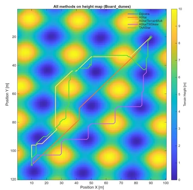
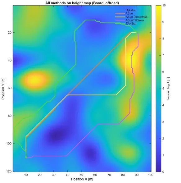
 Figures 5 and 6 compare the paths generated by all evaluated methods on Board_dunes and Board_offroad, respectively. The route overlays illustrate that incorporating additional terrain characteristics into the planning process can result in longer paths that avoid regions associated with high traversal costs. Consistent with the shared-cost evaluation, T-AAA* achieves balance between path length and terrain-related costs in both scenarios by avoiding steep slopes and favoring areas with lower traversal costs.

Board_mountain_pass represents a complementary case. On this map, the geometry of the terrain  strongly limits the set of feasible solutions, and the decision is therefore guided primarily by the directional elevation conditions. Accordingly, Table 2 shows identical best shared costs for the pitch/roll-aware planner and for the full T-AAA* planner on this map.

Figure 5: Height map of Board_dunes with the paths of all benchmarked methods

Figure 6: Height map of Board_offroad with the paths of all benchmarked methods

Discussion and Conclusions

The presented benchmark demonstrates that the primary contribution of the current implementation lies not in modifying the global A* search mechanism, but in redefining the local traversal cost through the integration of multi-layer terrain information and direction-dependent elevation penalties. This distinction is important for proper interpretation of the method. T-AAA* should not be viewed as a universal replacement for search-based planners; instead, it represents a terrain-aware extension of A* whose advantages become evident when the planning objective explicitly accounts for surface properties and slope-related traversal constraints.

The experimental results further indicate that purely geometric planning is insufficient under such conditions. While both Dijkstra and A* operate efficiently on the inflated grid, their solutions incur significantly higher cost when evaluated under the terrain-aware objective. Partial extensions provide measurable improvements; however, only the full T-AAA* formulation consistently captures both surface preferences and direction-dependent traversal effects relative to the terrain gradient. At the same time, the results suggest that the relative importance of individual cost components varies across environments. Flat terrains are primarily influenced by surface-related costs, whereas environments such as mountain passes or dune-like structures benefit more strongly from directional elevation modeling.

Future work will extend the proposed algorithm toward the automatic acquisition of terrain information from GIS (geographic information systems) data and its integration into a complete planning pipeline. In such a framework, the height map will be used to compute 3D distances as well as pitch- and roll-related terrain descriptors, while topographic object layers will provide information about terrain type and traversability. Future developments will also consider weather-related factors in order to predict terrain modifiers more realistically.

Overall, the study provides a consistent and implementation-aligned validation of the proposed method. The T-AAA* formulation achieves the lowest mean shared terrain-aware cost across all benchmark datasets, while maintaining favorable stability-related characteristics. These findings support the conclusion that combining direction-dependent elevation penalties with surface-based cost modeling is essential for effective path planning in complex, heterogeneous terrain.

References

• AbuJabal, N., Baziyad, M., Fareh, R., Brahmi, B., Rabie, T. and Bettayeb, M. (2024) ‘A comprehensive study of recent path-planning techniques in dynamic environments for autonomous robots,’ Sensors, 24 (24), 8089.
• Benrabah, M., Orou Mousse, C., Randriamiarintsoa, E., Chapuis, R. and Aufrère, R. (2024) ‘A review on traversability risk assessments for autonomous ground vehicles: methods and metrics,’ Sensors, 24 (6), 1909.
• Beycimen, S., Ignatyev, D. and Zolotas, A. (2023) ‘A comprehensive survey of unmanned ground vehicle terrain traversability for unstructured environments and sensor technology insights,’ Engineering Science and Technology, an International Journal, 47, 101457.
• Carvalho, A. E., Portugal, D. and Peixoto, P. (2025) ‘On terrain traversability analysis in unstructured environments: recent advances in forest applications,’ Intelligent Service Robotics, 18 (2), 195-213.
• Dijkstra, E. W. (1959) ‘A note on two problems in connexion with graphs,’ Numerische Mathematik, 1, 269-271.
• Ferguson, D. and Stentz, A. (2006) ‘Using interpolation to improve path planning: the Field D* algorithm,’ Journal of Field Robotics, 23 (2), 79-101.
• Hart, P. E., Nilsson, N. J. and Raphael, B. (1968) ‘A formal basis for the heuristic determination of minimum cost paths,’ IEEE Transactions on Systems Science and Cybernetics, 4 (2), 100-107.
• Koenig, S. and Likhachev, M. (2002) ‘D* Lite,’ Proceedings of the 18th AAAI Conference on Artificial Intelligence (AAAI ’02), 476-483.
• Likhachev, M., Ferguson, D., Gordon, G., Stentz, A. T. and Thrun, S. (2005) ‘Anytime Dynamic A*: an anytime, replanning algorithm,’ Proceedings of the 15th International Conference on Automated Planning and Scheduling (ICAPS ’05), 262-271.
• Likhachev, M., Gordon, G. J. and Thrun, S. (2003) ‘ARA*: anytime A* with provable bounds on suboptimality,’ Advances in Neural Information Processing Systems, 16, 767-774.
• Liu, Z., Guo, S., Yu, F., Hao, J. and Zhang, P. (2024) ‘Improved A* algorithm for mobile robots under rough terrain based on ground trafficability model and ground ruggedness model,’ Sensors, 24 (15), 4884.
• Nash, A., Daniel, K., Koenig, S. and Felner, A. (2007) ‘Theta*: any-angle path planning on grids,’ Proceedings of the AAAI Conference on Artificial Intelligence (AAAI-07), 1177-1183.
• Nishishita, T. and Ishigami, G. (2025) ‘Slip estimation model for traversability-based motion planning of cargo rover on extraterrestrial surface,’ Frontiers in Robotics and AI, 12, 1638667.
• Pohl, I. (1970) ‘Heuristic search viewed as path finding in a graph,’ Artificial Intelligence, 1 (3-4), 193-204.
• Sakayori, G. and Ishigami, G. (2024) ‘Modeling of slip rate-dependent traversability for path planning of wheeled mobile robot in sandy terrain,’ Frontiers in Robotics and AI, 11.
• Sánchez-Ibáñez, J. R., Pérez-del Pulgar, C. J., Serón, J. and García-Cerezo, A. (2023) ‘Optimal path planning using a continuous anisotropic model for navigation on irregular terrains,’ Intelligent Service Robotics, 16, 19-32.
• Stentz, A. T. (1994) ‘Optimal and efficient path planning for partially-known environments,’ Proceedings of the IEEE International Conference on Robotics and Automation (ICRA), Vol. 4, 3310-3317.
• Tang, Y., Zakaria, M. A. and Younas, M. (2025) ‘Path planning trends for autonomous mobile robot navigation: a review,’ Sensors, 25 (4), 1206.
• Waga, A., Benhlima, S., Bekri, A., Abdouni, J. and Saber, F. Z. (2025) ‘A survey on autonomous navigation for mobile robots: from traditional techniques to deep learning and large language models,’ Journal of King Saud University Computer and Information Sciences, 37, 198.
• Wang, N., Li, X., Suo, Z., Fan, J., Wang, J. and Xie, D. (2024) ‘Traversability analysis and path planning for autonomous wheeled vehicles on rigid terrains,’ Drones, 8 (9), 419.
• Xuan, D. T., Hung, N. T. and Thang, V. T. (2025) ‘A comprehensive review of improved A* path planning algorithms and their hybrid integrations,’ Automation, 6 (4), 52.