Jesús Fernando BEJARANO AUQUI1, Pedro Armengol GONZALES URBINA2 and
José NUÑEZ GALAVIZ2
1Universidad Peruana Unión, Lima, Perú
2Universidad de Montemorelos, México
Volume 2026,
Article ID 331210,
IBIMA Business Review,
13 pages,
DOI: doi.org/10.5171/2026.331210
Received date: 7 April 2026; Accepted date: 29 September 2026; Published date: 20 November 2026
Cite this Article as:
Jesús Fernando BEJARANO AUQUI, Pedro Armengol GONZALES URBINA and José NUÑEZ GALAVIZ (2026)," “ Optimizing Sales Forecasting using Time Series Models: Evidence from Alimentos del Norte Mexicano “, IBIMA Business Review, Vol. 2026 (2026), Article ID 331210, https://doi.org/10.5171/2026.331210
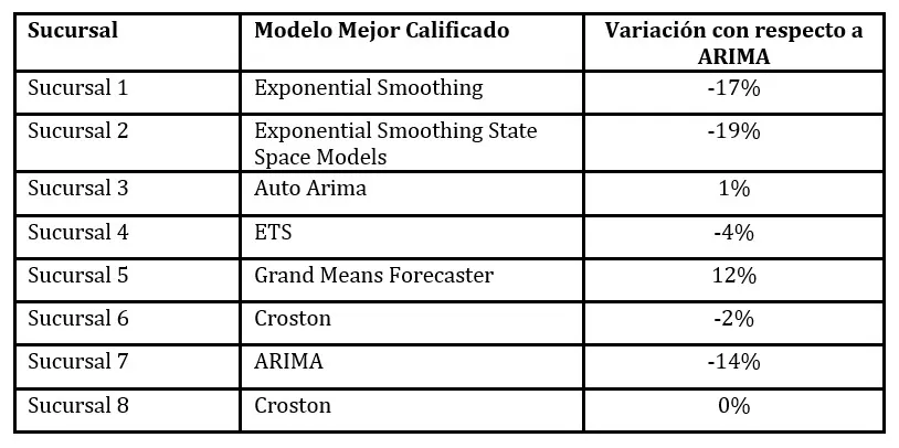
Accurate sales forecasting is essential for improving financial planning and inventory management in food industry companies. The motivation for this study stems from the diverse sales series behaviors observed across different branches, which complicates the selection of forecasting methods that deliver consistent performance. Furthermore, a gap exists in the literature regarding the limited number of studies that systematically compare multiple time-series techniques across the varying sales patterns found in food companies. To address this gap, the study evaluates twenty-eight forecasting models to project monthly sales for a Mexican food company for the year 2025. Regarding the methodology, historical data from eight branches were analyzed using various error metrics. The process followed the CRISP-DM framework and included models from the ARIMA, exponential smoothing, and Croston families, among others. Finally, the results revealed performance differences based on the specific characteristics of each sales series. ARIMA models performed best for branches 3 and 7; exponential smoothing for branches 1 and 2; and Croston for branches 6 and 8. The ARIMA model applied to branch 7 demonstrated the best relative performance, outperforming the other models considered by a margin of 14%. These findings support a differentiated approach to model selection based on the characteristics of each sales series.
Introduction
In the business world, time series analysis using mathematical and statistical models is essential for interpreting organizational behavior and supporting strategic decision-making, particularly in areas such as sales forecasting, inventory management, and financial planning. The sequential study of data facilitates the detection of trends and patterns, enabling the anticipation of demand and the optimization of resources—key factors for effective management. Furthermore, time series analysis reveals underlying relationships between variables across various sectors, reinforcing its analytical importance (Hyndman & Athanasopoulos, 2018). Thus, mathematical models help represent real-world situations and provide a basis for decisions regarding revenue, costs, sales, and operations (Render et al., 2012).
In the economic sphere, the use of time series is common for examining the evolution of indicators such as stock prices or unemployment rates. A thorough analysis of available information allows for the selection of the most appropriate methods and statistics for each case. This process relies on statistical techniques to model chronological data sequences and describe system behavior through stochastic processes, typically defined at regular time intervals (Shumway & Stoffer, 2006; Madsen, 2007). In the pursuit of profitability, companies employ time series analysis to anticipate future sales behavior based on historical data, thereby facilitating informed decision-making. Various studies have shown that forecast accuracy depends on the method used, the quality and time horizon of the analyzed data, and the ability to minimize errors. In the agricultural sector, as well as in business and auditing contexts, tools such as linear regression, ARIMA models, and other statistical models are used to identify trends and improve financial and operational planning (Corella et al., 2023; Prokofieva, 2022).
The objective of this research is to evaluate and select the most suitable time-series model for each branch in order to improve the accuracy of sales forecasts at Alimentos del Norte Mexicano1. Consequently, this research seeks to identify the best-performing forecasting model for the various branches analyzed, thereby contributing to more accurate decision-making and efficient management of the company’s resources.
Time Series
Time series analysis plays a fundamental role in financial forecasting. Various examples demonstrate how the application of these methods has enabled companies across different sectors to achieve significant savings and increase revenue through more accurate forecasts and efficient resource management as seen in cases such as Taco Bell, NBC, and Continental Airlines (Render et al., 2012). In the agricultural sector, the use of time-series-based approaches facilitates better financial planning. The choice of the most suitable method is determined by factors such as data availability and scope, model fit, and error minimization, as noted by (Corella et al., 2023).
In economics, time series are widely used tools for analyzing the evolution of data such as stock prices or unemployment rates. A rigorous analysis of the available information enables the selection of the most appropriate methods and statistics for each case. This approach relies on statistical methods to model ordered sequences of observations and describe system behavior through stochastic processes, typically defined at regular time intervals (Shumway and Stoffer, 2006; Madsen, 2007).
In the pursuit of profitability, companies turn to time-series analysis to anticipate future sales behavior based on historical data, thereby facilitating informed decision-making. Research has shown that forecast accuracy depends on the method employed, the quality and timeframe of the data analyzed, and the ability to minimize errors. Across the agricultural sector, as well as in business and auditing contexts, tools such as linear regression, ARIMA, and other statistical models are used to identify trends and improve financial and operational planning (Corella et al., 2023; Prokofieva, 2022).
In the fields of macroeconomics and finance, where data are typically organized as time series, there is a recognized need to refine analytical methodologies in order to understand both dynamic effects and long-term structural changes. In this context, time series are understood to be composed of elements such as trend, cycle, seasonality, and irregularity; the interaction among these components explains the evolution of the data and underpins their analysis and modeling (Cochrane, 1997; Stock & Watson, 2017; Anderson et al., 2011).
Thus, time series analysis has historically played a fundamental role in various scientific and business fields, where traditional parametric approaches have been widely applied. Increased data availability and the development of new computational capabilities have enabled improved modeling of temporal dynamics, establishing advanced statistical tools as an essential component of modern forecasting models (Bryam Lim, 2021).
Forecasting Models
(Reid and Sanderes, 2011) note that forecasting plays a crucial role in business operations, as decisions across all functional areas rely on future predictions. Areas such as markets, products, inventories, and human resources require forecasting, which is why companies invest heavily in technologies that facilitate better future planning. It is unlikely that any event is entirely predictable, as unknown factors-such as unexpected changes in wind speed that might slightly alter a missile’s trajectory-can arise and affect its course. In many instances, it is necessary to address a phenomenon that evolves over time such as a newspaper’s monthly sales where multiple unknown variables are at play, making it difficult to establish a deterministic model that accurately predicts future behavior. However, it is feasible to develop a model that calculates the probability of a future value falling within specific limits; this type of model is known as a probabilistic or stochastic model (Newnan et al., 2016). Commonly used quantitative models include time series decomposition, exponential smoothing, and methods such as regression, autoregression, and autoregressive integrated moving average (ARIMA). These methods are supported by a rigorous statistical framework,
Alimentos del Norte Mexicano is a fictitious name used to preserve the confidentiality of the participating company. The sales figures and business information presented are real; only the company’s name has been replaced.
And, among them, the ARIMA model has proven to be the most effective in terms of modeling performance (Corres et al., 2014).
Autoregressive Integrated Moving Average (ARIMA)
ARIMA models are particularly reliable for short-term forecasting, as most ARIMA models place significant emphasis on the recent past rather than the distant past (Pankratz, 1983). In these models, the variable of interest, Y, is estimated using a linear combination of past values (autoregressive component) and/or past forecast errors (moving averages). (Box et al., 2016), and Hyndman and Athanasopoulos (2018) provide the theoretical foundation for developing time series models, specifically examining ARIMA model theory. Furthermore, they review methods for estimating model coefficients, selecting the most appropriate model, and generating forecasts. A time series is considered a stochastic or random process consisting of a collection of random variables (Y1, Y2, …, YN) ordered in time (T1, T2, …, TN) that satisfy stationarity meaning the mean (μ), variance (σ), and autocovariance (γ) are constant (Box et al., 2016), such that each point is independent of the others.
Croston (CRO)
Croston was one of the first researchers to point out that applying traditional exponential smoothing methods led to significant forecasting errors for intermittent demand. The Croston method (CRO) is based on simple exponential smoothing but splits the time series into two parts: the first consists of a series of positive demand values, while the second contains the time intervals between consecutive non-zero demands. A forecast is calculated for each of these series using exponential smoothing, and both values are subsequently updated whenever a non-zero demand occurs (Croston, 1972).
Exponential smoothing
Smoothing methods provide a class of time series models that reduce the random variation within a time series, thereby revealing the underlying process signal. A variety of smoothing models are presented; these either continuously average the series over a moving interval of observed values or fit a polynomial approximation to a restricted segment of the series. Among the available smoothing techniques, the exponential smoothing model has proven useful due to its simplicity of application (Brown, 1956).
Exponential smoothing state-space models (ETS)
According to (Hyndman et al., 2008), exponential smoothing methods originated in the 1950s and remain the most widely used forecasting approaches in business and industry. The ETS (Exponential Smoothing State-Space Models) approach provides a statistical framework while preserving the intuitive nature of exponential smoothing.
Grand Mean Forecaster
(Box et al., 1970) note that the Grand Mean Forecaster is a time-series forecasting method based on calculating the mean of all data available up to that point as the prediction for the next period. It is a simple approach that assumes the past trend of the data is representative of future behavior.
Error Metrics
It is essential to consider the error inherent in any prediction. Various studies, such as that by (Chu and Zhang, 2003), highlight the importance of this aspect in decision-making. Ignoring prediction error can have unintended consequences across all areas of a company. According to information provided by IBM (n.d.), statistical analysis employs several accuracy measures, such as MAE (Mean Absolute Error), MASE (Mean Absolute Scaled Error), percentage accuracy, RMSE (Root Mean Squared Error), and MAPE (Mean Absolute Percent Error). These measures are based on historical data and can serve as indicators of forecast accuracy. For instance, MASE is calculated by dividing the model’s MAE by the MAE of the naïve model, allowing for an assessment of the model’s relative accuracy compared to a simple benchmark model. Additionally, other error metrics are explained such as MSE (Mean Squared Error) and its square root, RMSE which provides insight into the dispersion of errors between fitted and observed values.
Methodology
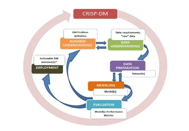
The research employed a quantitative approach and a non-experimental longitudinal design. Given that data analysis projects whether in academia or industry share fundamental data mining principles, various methodologies have been formulated to standardize these processes, differing in the depth of their stages and their specific applications (Bakumenko & Elragal, 2022). Among the most recognized are SEMMA, KDD, and CRISP-DM (Plotnikova et al., 2020).
The CRISP-DM methodology was selected for this study because it offers a systematic, iterative structure, prioritizes understanding the business context, and adapts to dynamic financial environments, thereby facilitating efficient project management. The process began with an understanding of the financial operations and objectives of a food company in Mexico. Subsequently, sales time series data covering the period from January 2015 to February 2025 were analyzed and prepared.
Next, various time series models were constructed and compared using PyCaret in Python. Training data from 2015 to 2023 and testing data from 2023 to 2025 were used for this purpose. These models were evaluated using various error and goodness-of-fit metrics to identify the most accurate one. Finally, the selected model was used to generate monthly sales forecasts from March to December 2025, aiming to support financial planning and decision-making.
Fig 1. Continuous process cycle for the CRISP-DM methodology
The study was conducted at Alimentos del Norte Mexicano, a Mexican company dedicated to the production and marketing of food products, specializing in vegetarian items and plant-based food alternatives. The organization operates primarily in Northern Mexico within the food and beverage sector, specifically focusing on the segments of vegetarian foods, plant proteins, and soy-based products. Its scope of operations encompasses production, marketing, and distribution activities aimed at both the consumer market and business clients within the food industry and foodservice sector.
The company’s product portfolio includes plant-based proteins, meat alternatives, beverages, cereals, and other soy-based nutritional products. This product diversity entails addressing varied consumer needs and managing commercial categories with potentially distinct demand characteristics. Regarding sales channels, the company sells through its own stores, distributors, direct sales representatives, and business-to-business supply channels. Consequently, its commercial operations encompass both sales to end consumers and transactions with business clients, introducing distinct purchasing patterns and commercial planning requirements.
Founded in the 1950s, Alimentos del Norte Mexicano has a workforce of approximately 400 to 500 employees. This study utilized historical sales records from eight branches located in northern Mexico. Selecting these units allows for an examination of sales performance within a real-world operational context and an evaluation of the utility of time-series models in generating forecasts to support business planning. The geographic scope of the analysis is limited to the branches included in the study; therefore, the results must be interpreted in the context of the specific operations and data analyzed, without necessarily assuming they represent the organization’s entire range of activities.
From a competitive standpoint, the company operates in a segment of the food market where plant-based alternatives compete with other food options and products from various brands and manufacturers. However, it was not possible to establish a verifiable estimate of its market share within the analyzed geographic and commercial segment due to a lack of publicly available, disaggregated data regarding the company’s total sales and the size of the relevant market. Consequently, the study does not assign the organization a specific competitive position, nor does it present a market share figure that cannot be empirically substantiated.
In this context, the variety of products sold, the coexistence of different sales channels, and the geographical distribution of branches make it relevant to have forecasting tools capable of identifying temporal patterns and anticipating demand trends. The application of time series models can help improve sales planning, inventory management, sourcing decisions, and the allocation of commercial resources. Therefore, Alimentos del Norte Mexicano serves as the organizational setting for evaluating the ability of these models to optimize sales forecasting based on historical data from eight branches.
The study population consisted of all historical sales records for the company’s flagship product during the period from January 2015 to February 2025. A total of 880 observations were collected, comprising 110 monthly observations for each of the eight branches analyzed. The study variable sales volume is quantitative in nature and is expressed using decimal numerical values. Data were obtained from a local database hosted on Microsoft SQL Server and provided by the food company. This source provided access to the historical records required for the analysis, with the integrity and consistency of the data being taken into account during the data preparation process. Jupyter Notebook was used for time-series modeling and evaluation, while Power BI was employed to visualize the results and facilitate their interpretation by company management.
The study began with the retrieval and consolidation of historical sales data from eight branches, using backups restored to a database server. Subsequently, records were extracted via SQL queries and integrated into a CSV file for processing and analysis. The data were then imported into and prepared within the Jupyter Notebook environment using Python and the PyCaret library. Based on this foundation, time-series models were applied to analyze sales behavior and identify patterns, trends, and seasonal components. The models were evaluated against one another to select those offering the best predictive performance. Finally, the selected models were used to generate sales forecasts for the next ten months for each of the eight branches. The results were exported to a CSV file to facilitate review, visualization, and use in supporting sales planning and strategic decision-making.
Results
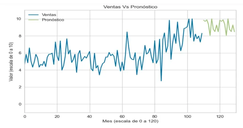
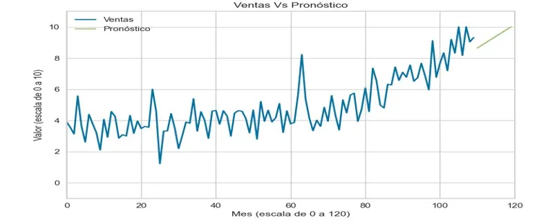
Figure 2 displays the historical sales for Branch 1 and the forecasts generated for the branch over a 120-month period, revealing a clear relationship between actual data and future projections. Historical sales show an upward trend over time, albeit with marked fluctuations reflecting peaks and dips at various points. From month 100 onwards, sales appear to stabilize at values close to 9 or 10, indicating potential seasonal behavior or a growth ceiling. The results demonstrate that Branch 1 has reached a point of sales stability, and the forecasts align with this pattern. This provides a solid foundation for planning maintenance strategies, although it would be prudent to explore opportunities to drive further growth through innovations or new marketing campaigns. The forecast line shows high stability, suggesting that Branch 1 has reached a stage of operational maturity. This is attributable to factors such as customer loyalty, market consolidation, or a balance between supply and demand.
Fig 2. Sales and forecast generated for branch 1
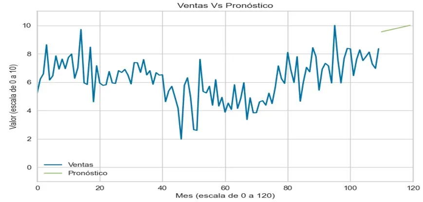
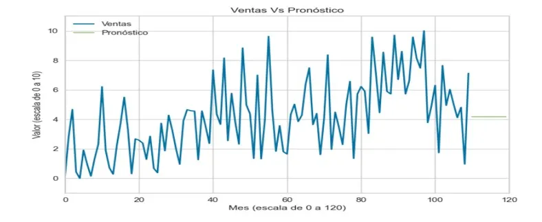
Figure 3 shows that sales at Branch 2 fluctuate significantly over time, exhibiting periods of high variability and a general upward trend, particularly after month 60. The green forecast line indicates a continuation of the upward trend observed in historical sales data. This implies that, according to the model used, future sales will continue to rise due to factors such as increased demand, customer loyalty, or effective commercial strategies. The branch is demonstrating positive sales performance, and the forecasting model projects stable growth. This may suggest that the strategies implemented are effective or that there is growing market demand.
Fig 3. Sales and forecast generated for branch 2
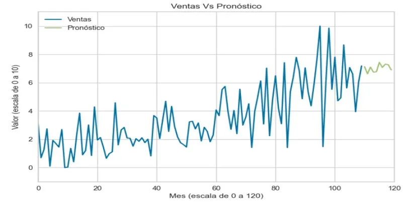
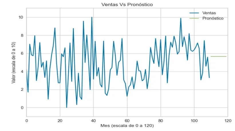
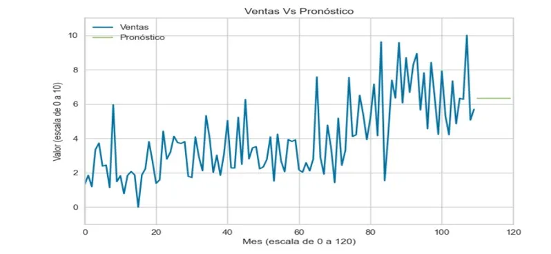
Figure 4 shows actual sales exhibiting an upward trend with significant fluctuations, particularly toward the second half of the period. However, from month 100 onwards, there is a noticeable decrease in peak values, which could be linked to internal or external factors affecting sales dynamics. Secondly, the model generates a constant forecast close to the average sales value approximately 6 towards the end of the period. This indicates that while the model is designed to capture general behavior, it fails to reflect the fluctuations observed in actual sales. Thirdly, the model has limitations; although the forecast provides a reasonable general idea of sales levels, it does not account for oscillations or the drop in recent peak values. This may limit its utility for tactical decisions, such as inventory management or specific promotions. Fourthly, the figure reveals a discrepancy between actual sales and the forecast that is most evident in the final months, where the model underestimates peak values and fails to adapt to sales variations. This suggests that the model does not adequately incorporate recent changes or more complex trends. The analysis indicates that the forecast for Branch 3 offers a basic level of estimation useful for general or long-term analysis but is insufficient to capture the fluctuations and shifting dynamics observed in actual sales. Implementing a more robust model that incorporates trends and seasonal variability would be advisable.
Fig 4. Sales and forecast generated for branch 3
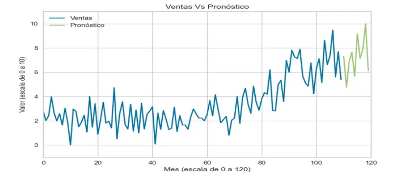
Figure 5 shows a predictive pattern that is sustained over time, albeit with significant fluctuations during certain periods. From month 100 onwards, values approach the upper limit of the scale (10), indicating a potential period of high demand. Secondly, the forecast displays an upward trend toward the end of the period, aligning with overall sales behavior. This model effectively captures the global trend, suggesting it correctly incorporates the growth observed in historical data. Thirdly, the model’s predictive capability appears particularly accurate for this branch, as it reflects both the upward trend and the projected values for the final months. However, it fails to capture specific, localized fluctuations seen in actual sales—particularly sharp peaks or drops. Fourthly, the forecast is useful for medium- and long-term decision-making—such as resource planning, inventory management, and growth strategies—because it reflects the sustained trend of rising sales. Overall, the forecast for Branch 4 is effective at capturing the upward sales trend, thereby enabling reliable strategic planning. Nevertheless, to maximize its utility, it would be necessary to incorporate elements that better reflect short-term fluctuations.
Fig 5. Sales and forecast generated for branch 4
Figure 6 shows actual sales (blue line) and forecasts (green line) for Branch 5 over a 120-month period. Sales are quite volatile, exhibiting marked fluctuations. These variations could stem from seasonal factors, changes in demand, or specific events at the branch. A second key observation concerns the behavior of the forecast (green line), which reveals significant implications for Branch 5 specifically, the model’s lack of adaptability. Furthermore, the forecast fails to reflect the significant fluctuations seen in actual sales. Instead of tracking the observed volatile patterns, it remains at a constant level, demonstrating that the model is capturing neither the seasonality nor the trends inherent to the branch’s operational reality.
Fig 6. Sales and forecast generated for branch 5
Figure 7 illustrates the behavior of actual sales and the forecast for branch 6 over a 120-month period. First, actual sales exhibit considerable fluctuations, yet the trend is more moderate compared to other branches. While there are recurring peaks and dips, they are not extreme, suggesting a degree of relative stability. Second, the forecast shows a constant value (close to 4.5) that fails to respond to the changes observed in actual sales. This indicates that the model employed likely relies on a historical average or a basic technique, without accounting for seasonality, trends, or data variability. The figure demonstrates that the forecast for branch 6 remains constant and does not reflect actual sales fluctuations, indicating a model poorly adapted to the business’s dynamics.
Fig 7. Sales and the forecast generated for branch 6
The most favorable evaluation was obtained with ARINA; the graphical illustration of the forecast in figure 8 highlights the following points: First, there is an upward trend in actual sales over time, albeit with fluctuations. This may reflect a steady rise in demand combined with occasional spikes and dips caused by seasonal factors or specific events. Second, there is initial stability followed by acceleration; during the early months, actual sales remain relatively stable with moderate fluctuations. From the second half of the period onward, more rapid growth is observed, indicating a shift in business dynamics (possibly due to factors such as expansion strategies, promotional activities, or increased demand). Third, there is a progressive adjustment of the forecast as the model’s accuracy improves over time. In the initial months, the forecast does not track sales fluctuations closely, but, towards the end of the period, it aligns significantly with the upward trend. This suggests that the model relies on accumulated data to refine its predictions—an approach that can be useful for clear trends but less effective during initial periods.
Fig 8. Sales and the forecast generated for branch 7
Figure 9 demonstrates that the Croston model, the one primarily evaluated, reveals significant variability in actual sales throughout the period, characterized by notable peaks and drops. Although sales tend to rise moderately over time, the data do not show uniform growth, suggesting that external or internal factors are driving these fluctuations. Secondly, the model generates a constant forecast toward the end of the period, hovering around a value of 6; this indicates that the model relies on a historical average for its predictions, disregarding the trends and fluctuations observed in actual sales. Thirdly, the model fails to capture sales peaks and drops, demonstrating an inability to reflect seasonal patterns or specific variations. This can negatively impact branch planning, particularly regarding inventory management and sales strategies. Finally, the discrepancy between actual sales and the constant forecast could lead to operational issues such as overstocking or stockouts during periods of high demand as well as lost revenue opportunities. The figure illustrates high variability in actual sales alongside a forecast that fails to align with these dynamics, highlighting the need to improve the model to support more accurate, strategic decision-making.
Fig 9. Sales and forecast generated for branch 8
Models belonging to the ARIMA family are an important tool used in time series analysis and forecasting. This study compared these models to quantify the percentage deviation from the best-performing model, using error metrics as the criterion. For branches 3 and 7, the comparison was made against the second-best model, as the optimal model exhibited anomalous behavior. The analysis was based on average sales observed during the period from January 2015 to February 2025 (table 1)
Table 1. Average sales
Based on the analysis of Figures 1 through 8, it is concluded that the model corresponding to Branch 7 demonstrates the best performance in representing actual sales versus the generated forecast. This result is supported by the model’s ability to adequately capture the series’ general trend reflecting sustained sales growth toward the end of the analyzed period even though it does not fully replicate specific point-in-time fluctuations. This is due to the following reasons:
The model for Branch 7 demonstrates greater consistency in recent months, showing a more precise alignment between observed and estimated values. This behavior indicates effective learning of the underlying data structure and superior predictive stability compared to the other branches evaluated.
Consequently, this model stands out as the most suitable for supporting medium and long-term strategic planning, as it incorporates a trend consistent with actual sales performance. In contrast, the models for Branches 3 and 8 show limited performance by relying on virtually constant forecasts, which reduces their ability to capture relevant dynamics within the series. Overall, the results confirm the superiority of the Branch 7 model as the most robust and reliable option for decision-making.
Discussion
The purpose of this study was to evaluate eight models to identify the most efficient ones for sales forecasting across eight branches of a food company located in northern Mexico. The results indicate that there is no single model universally applicable to all datasets, as the forecasting process is inevitably subject to uncertainty and the influence of external factors. These findings align with (Rubwurm et al., 2020), who highlight that while predictive models are valuable tools for anticipating future scenarios and detecting deviations from expected behavior, forecasts entail a degree of uncertainty, and no estimate is free from error. Similarly, (Assad et al., 2022) emphasize that causal analysis and discovery in time series represent a rapidly evolving field of research; new methods constantly emerge, and no single family of approaches is superior in all circumstances, as each relies on assumptions that may not hold true for every dataset. Likewise, (Zhang et al., 2014) demonstrated through the analysis of various time series models and error metrics such as MAE, MAPE, and MSE that no single method consistently outperforms the others. Specialized literature indicates that classical time-series models, such as ARIMA and ETS, can deliver adequate performance; however, their effectiveness is heavily dependent on the context and the specific characteristics of the data being analyzed. (Schaffer et al., 2021) note that selecting the most appropriate ARIMA model can be a complex and sometimes subjective process, although automated tools like auto.arima have helped simplify this task. On the other hand, (Huadsri and Phaphan, 2024) and (Jain and Mallick, 2017) demonstrate that linear models can outperform non-linear approaches when the relationships between variables are stable and well defined, achieving competitive results when evaluated using metrics such as MAE, MASE, MAPE, and RMSE. However, (Reich et al., 2016) highlight that model performance varies according to the forecast horizon: baseline models based on recent observations tend to be more effective in the short term, whereas incorporating long-term components does not always yield significant improvements. Consistent with these findings, the results obtained in this study confirm that there is no single dominant model for all branches, underscoring the importance of selecting a specific model for each series and time horizon.
Conclusion
Twenty-eight time-series models applied to the sales of a food company’s flagship product in northern Mexico were evaluated, using data spanning from January 2015 to February 2025. Model comparison was conducted using error metrics such as Mean Absolute Percent Error (MAPE), Root Mean Squared Error (RMSE), Mean Squared Error (MSE), Mean Absolute Scaled Error (MASE), and Mean Absolute Error (MAE). Regarding forecasts for the months of March through December 2024 across the eight analyzed branches, two ARIMA-family models yielded the best results for branches 3 and 7; exponential smoothing performed best for branches 1 and 2, while the Croston model excelled for branches 6 and 8. These results suggest that each dataset in this case, each branch may require a different forecasting model due to the specific characteristics of its records. Furthermore, the most suitable model for a given branch might change over future periods. The diversity of optimal models identified highlights the need for individualized time-series analysis for each branch, avoiding generalizations that could compromise forecast accuracy. Additionally, periodic model re-evaluation and forecast adjustments are recommended as new data becomes available, given that both market conditions and consumer behavior can shift over time.
References
Anderson, D. R., Sweeney, D. J., Williams, T. A., Camm, J. D. y Martin, K. (2011). Métodos cuantitativos para los negocios, (11a ed.).
Assaad, C. K., Devijver, É. y Gaussier, É. (2022). Survey and evaluation of causal discovery methods for time series. The Journal Of Artificial Intelligence Research, 73, 767-819. https://doi.org/10.1613/jair.1.13428
Bakumenko, A. y Elragal, A. (2022). Detecting anomalies in financial data using machine learning algorithms. Systems, 10(5), 130. https://doi.org/10.3390/systems10050130.
Box, G., Jenkins, G. y Reinsel, G. C. (1970). Time series analysis: forecasting and control. Holden-Day.
Box, G., Jenkins, G., Gregory, R. y Greta, L. (2016). Time series analysis: forecasting and control. Wiley.
Brown, R. G. (1956). Exponential smoothing for predicting demand. Cambridge.
Bryan Lim, S. Z. (2021). Time-series forecasting with deep learning: a survey. Royal Society Publishing, 1-14. https://doi.org/10.1098/rsta.2020.0209
Chu, C. W. y Zhang, G. P. (2003). A comparative study of linear and nonlinear models for aggregate retail sales forecasting. International Journal Of Production Economics, 86(3), 217-231. https://doi.org/10.1016/s0925-5273(03)00068-9
Cochrane, J. H. (1997). Time series for macroeconomics and finance. University of Chicago.
Corella, J., Rusnak, J., Binns, J., Rovira, C., Ayala, O., Ríos, R. y Vargas, E. (2023). Evaluation of five methods for forecasting and analysis of agricultural production trends in Panama: a tool for institutions and companies in the sector. Revista Investigaciones Agropecuarias, 16-27.
Corres, G., Passoni, L. I., Zárate, C. y Esteban, A. M. (2014). Estudio comparativo de modelos de pronóstico de ventas. Iberoamerican Journal Of Industrial Engineering, 6(11), 113-134. https://doi.org/10.13084/2175-8018/ijie.v6n11p113-134
Croston, J. D. (1972). Forecasting and stock control for intermittent demands. Journal of the Operational Research Society, 23(3), 289-303. https://doi.org/10.1057/jors.1972.50
Huadsri, S. y Phaphan, W. (2024). The development of forecasting models for life insurance data by employing time-series analysis and machine learning technique. WSEASTransactions OnMathematics, 23, 196-205. https://doi.org/10.37394/23206.2024.23.23
Hyndman, R. J. y Athanasopoulos, G. (2018). Forecasting: principles and practice (2a. ed.).
Hyndman, R., Koehler, A., Ord, K. y Snyder, R. (2008). Forecasting with exponencial smoothing. The State Space Approach.
Jain, G., y Mallick, B. (2017). A Study of Time Series Models ARIMA and ETS. Social Science Research Network. 1, 1-7. https://doi.org/10.2139/ssrn.2898968
Madsen, H. (2007). Time series analysis. Tylor y Francis Group.
Newnan, D. G., Eschenbach, T. G., & Lavelle, J. P. (2012). Engineering Economic Analysis.
Pankratz, A. (1983). Forecasting with univariate box‐Jenkins models: Concepts and cases. https://doi.org/10.1002/9780470316566
Plotnikova, V., Dumas, M. y Milani, F. (2020). Adaptations of data mining methodologies: a systematic literature review. Computer Science, 6(e267). https://doi.org/10.7717/peerj-cs.267
Prokofieva, M. (2022). Integrating data analytics in teaching audit with machine learning and artificial intelligence. Education And Information Technologies,28(6), 7317-7353. https://doi.org/10.1007/s10639-022-11474-x
Reich, N. G., Lessler, J., Sakrejda, K., Lauer, S. A., Iamsirithaworn, S. y Cummings, D. A. T. (2016). Case study in evaluating time series prediction models using the relative mean absolute error. The American Statistician, 70(3), 285-292. https://doi.org/10.1080/00031305.2016.1148631
Reid, D. y Sanders, N. (2011). Operations management an integrated approach. John Wiley y Sons, Inc.
Render, B., Stair Jr, R. M. y Hanna, M. (2012). Métodos cuantitativos para los negocios. Pearson Educación.
Rubwurm, M., Ali, M., Zhu, X. X., Gal, Y., y Körner, M. (2020). Model and Data Uncertainty for Satellite Time Series Forecasting with Deep Recurrent Models. IEEE. https://doi.org/10.1109/igarss39084.2020.9323890
Schaffer, A. L., Dobbins, T. y Pearson, S. (2021). Interrupted time series analysis using autoregressive integrated moving average (ARIMA) models: a guide for evaluating large-scale health interventions. BMC Medical Research Methodology, 21(1).58-61. https://doi.org/10.1186/s12874-021-01235-8
Shumway, R. H. y Stoffer, D. S. (2006). Time series analysis and its applications. Springer.
Stock, J. H. y Watson, M. W. (2017). Twenty years of time series econometrics in ten pictures. The Journal Of Economic Perspectives, 31(2), 59-86. https://doi.org/10.1257/jep.31.2.59
Zhang, X., Zhang, T., Young, AA. y Li, X. (2014) Applications and comparisons of four time series models in epidemiological surveillance data. PLoSone,9(2): e88075. https://doi.org/10.1371/journal.pone.0088075