Nowcasting The Output Gap for Romania Using a Mixed-Frequency Approach

Introduction

The output gap is one of the most chased macroeconomic indicators by the central banks due to its significant relevance in the process of monetary policy decisions. The assessment of the stance of the business cycle and the potential evidence of an overheating economy is essential to cease with the upward pressures and to stabilize inflation. Technically, the output gap is computed as the difference between the potential level of the output and the actual one. Hence, the estimation of this indicator becomes challenging given its characteristic of being an unobservable component. Moreover, only the real output can be observed by the economists but it is published quarterly and becomes available with a delay of more than two months following the end of the reference period. Providing a reliable approach to assess this cyclical component of the real economy is crucial for monetary policy authorities in the transmission mechanism.

Estimating the real-time output gap and finding the “best” measure to describe the degree of slack in the economy is far more difficult than the classical decomposition of a time series into stochastic trend and stationary cycle. To be able to track the output gap closely within a quarter and after it, we have to use high-frequency data, an aspect that could induce more uncertainty due to incomplete observations for the recent past (‘ragged edge problem’, see Wallis (1986)), publication lags and data revisions. Thus, it becomes difficult for monetary policy to assess the cyclical position of the economy and to make rapid and timely appropriate interventions, especially in periods marked by unexpected demand and supply shocks, sudden regime changes in the economy, energy crises, such as the ones that appeared immediately after the COVID-19 pandemic or the war in Ukraine.

In this paper, we follow the approach proposed by Morley and Wong (2020) and Berger et al (2023) to estimate the real-time output gap. We accommodate the data set for Romanian characteristics and perform the assessment over the period 2003-2022. The model incorporates time series representative for a small open economy, most commonly used in the literature (in the absence of real-time GDP data) such as industrial production, turnover in retail trade and services, 3-month interest rate, consumer sentiment index and financial data. The importance of the output gap derives from the monetary policy authority’s objective of maintaining price stability. The Romanian economy was recently hit by the multitude of shocks associated with the COVID-19 pandemic outbreak and the vulnerabilities induced by the different variants of the coronavirus. Under these circumstances, the macroeconomic outlook becomes difficult to predict. The household’s consumption significantly decreases despite the implementation of social measures, while gross fixed capital formation posted positive average annual dynamics in 2020 as a whole. In 2021 and 2022, the fast-paced recovery was affected by the rise in energy prices, the surge in inflation, bottlenecks in global value chains and the war in Ukraine. Thus, the assessment of the cyclical position of the economy becomes more complex given the fact that the context is very uncertain and the data for real GDP was recently subject to multiple revisions from the National Institute of Statistics. The method used in this paper proved to be highly correlated with a simple univariate filter, while capturing a large negative output gap immediately after the outbreak of the Covid-19 pandemic and the strong rebound afterward. The trajectory in recent periods and the overheating of the economy may be also associated with persistent inflationary pressures in the economy.

Starting from the fact that the output gap is not directly observable in the literature, the proposed methods to assess this indicator rely on linear univariate filtering techniques. One of the most widely used is the basic Hodrick-Prescott (HP) filter (1997) which decomposes a time series into a cyclical component (gap) and a permanent one (trend) by minimizing the deviation of the observable from the trend as well as the curvature of the estimated trend. The trade-off between these two goals is given by a smoothing calibrated parameter. However, despite its prevalence, the criticism (see among others, Hamilton (2018)) shows that HP filter is not adequate for extracting the cyclical component of the real GDP from several reasons. This is a purely statistical method that it may induce spurious dynamics while it is not designed to capture the theoretical features of the underlying data-generating process. Moreover, it suffers from “end-of-sample” problems, meaning that the filtered values at the end of the sample are subject to revisions as the sample is extended with recent data. Moreover, Morley and Wong (2020) mention that using univariate models like filtration methods based only on a single variable which is decomposed in trend and cycle components requests for incorporating additional information outside the model to be corroborated with the results.

As discussed in detail in Woodford and Walsh (2006), for policy commitment, not only the price stability should matter, but also a stabilization in the “output gap” is justified. Therefore, other common techniques that were developed in estimating output gap have focused on multivariate filters. These add some economic structure through theoretical relationships such as Philips curve or Okun’s law and produce more reliable estimates than univariate techniques. Among them, we find the multivariate HP filter proposed by Laxton and Tetlow (1992), Beveridge and Nelson (1981) or Benes et al (2010). The last above mentioned represent a milestone in the literature related to the estimation of the potential output and the output gap by incorporating in a small model a set of relationships between actual and potential GDP, unemployment, core inflation and capacity in utilization in the manufacturing sector. Furthermore, the multivariate filter of Benes et al (2010) can deal with revisions of current estimates for the output gap as new information is incorporated in the data set. Afterwards, this approach was developed by Blagrave et al (2015), Alichi (2015) or Alichi et al (2017).

An extension of the class of univariate and multivariate filters for estimating the unobserved states of the economy is denoted by the unobserved component model (UCM) proposed by Harvey (1989). The model uses a multivariate set-up that relies on a state-space representation with an embedded production function, where the Kalman filter and smoother can be applied for state-space representation. This framework accounts for joint identification of trends and gaps in a single system of equations having a rich economic structure. In other words, this approach uses inter-dependencies not only across cyclical components but also across stochastic trends (see Tóth, 2021; Radovan, 2021). The Bayesian methods used for estimation help to overcome identification problems given the conditional posterior distribution obtained through a mixture between prior beliefs and the information in the data.

However, these unobservable estimates representative for the state of the economy are surrounded by a high degree of uncertainty and are subject to revisions as new data from national accounts become available. Regarding the data revisions’ problem, Orphanides and van Norden (2002) mention that historical data revisions may not be the main source for revision of the estimates, but rather they can happen due to pervasive unreliability of end-of-sample values. Moreover, sometimes changes in estimates that are derived from data revisions can be desirable as the new information reflects more properly the economic conditions. However, the UCM appears to have good revision properties and reasonable forecasting performance in terms of output gap due to the Kalman smoother algorithm (Tóth, 2021).

As for uncertainty, the main sources can be classified as i) filter uncertainty reflected by the nature of the underlying process of the unobservable states; ii) parameter uncertainty inherent in econometric models given the fact that the parameters of the state-space representation are unknown and need to be estimated; iii) model uncertainty which is a potential misspecification given the fact that models are an approximation of the reality and are based on a set of assumptions.  Taking into consideration all of these concerns, Bayesian methods may provide a straightforward method to quantify the modeling uncertainty and mitigate it.

New-Keynesian models as DSGE received great interest in recent years among technical methods to estimate the output gap and the potential output. The structure of these models is based on microeconomic foundations, providing from a theoretical point of view a much more rigorous method. Agents usually form rational expectations and maximize their objective function subject to some economic constraints. Moreover, these models are derived from optimal monetary policy theory and the results have a quantitative and structural interpretation of macroeconomic dynamics (see among others, Veltov et al 2011; Primiceri and Justiniano, 2009, Juillard et al, 2006).

Therefore, we find a vast methodology to estimate the output gap based on the historical data set. But there were little pieces of evidence when it comes to real-time estimate or nowcasting of the output gap. Several methods based on mixed-frequency analysis were implemented to nowcast the real GDP. Burlon and D’Imperio (2020) present a model-based measure having real-time DSGE estimates for the output gap, which is stable in time and less prone to ex-post revisions. A recently pseudo-real time analysis to estimate the euro area output gap through Beveridge-Nelson decomposition based on a large Bayesian vector autoregression is described by Morley et al (2022). This exercise that is very similar to Berget et al (2023) is conducted to address features associated with COVID-19 pandemic with the help of multivariate information coming from the unemployment rate or hours worked. Even if the evaluation sample is short, the model seems to perform well compared to the classical HP filter.

The rest of the paper is organised as follows. Section 2 describes the methodological approach that we use to conduct this analysis. In the next section, we present the data set and the results from the multivariate decomposition methods and the last section concludes the paper.

The Model

The approach proposed in this paper is based on the Beveridge-Nelson decomposition with a mixed-frequency Bayesian VAR described as in Berger et al (2023) and Morley and Wong (2020). According to Beverigde and Nelson (1981), any non-stationary time series can be decomposed into permanent and transitory components. On the one hand, the permanent component  follows a random walk with drift and it is defined by the difference between the long-run conditional expectations minus any deterministic future movements in time series. On the other hand, the transitory or the cyclical component  is defined as the difference by the actual value and the permanent component.

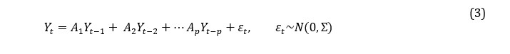
The vector process  includes all observed variables to estimate the trend component from eq. (1) and then to calculate cyclical component from eq. (2), is assumed to have a vector autoregressive structure with p lags VAR (p) at quarterly frequency:

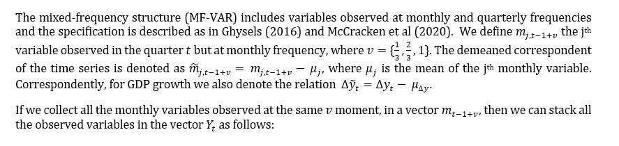
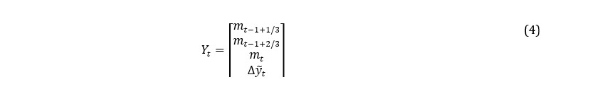
If we collect all the monthly variables observed at the same  moment, in a vector , then we can stack all the observed variables in the vector  as follows: 

For example, if we consider 2022Q4 and its previous quarter, then  is represented by

For    we can define the companion form of VAR (1) model

Where  is a vector of demeaned variables,  is the companion matrix, and  are residuals, linked to forecast errors through expression . The nowcasting problem that has to be addressed is related to how we can estimate given partial knowledge about . Therefore, the cyclical component of  (real GDP) can be calculated as follows

Where s_k is a vector having 1 at its k^th element (supposed to be included as real GDP growth Δγ_t ) and zero otherwise.

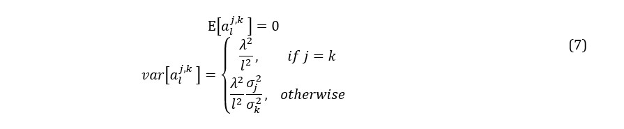
The Bayesian estimation procedure is based on Morley and Wong (2020). The method uses a natural conjugate prior with a standard Minnesota structure for implementing shrinkage in a Bayesian VAR model. We set the prior means and variances of the slope coefficient σ ^j,k of the l^th lag of variable k in the j^th equation of the VAR model in equation (3).

We set the parameter , representative for the degree of shrinkage in the BVAR, following Morley and Wong (2020) through numerical method by optimizing the one-step-ahead out of sample forecast for the output growth. If , the variables from the model are independent white noise processes, while for positive values of , the posterior will converge asymptotically to the population parameters. In this paper, we set the  parameter to optimize the one-step-ahead out-of-sample forecast of output growth so as to not overfit output growth with the model.

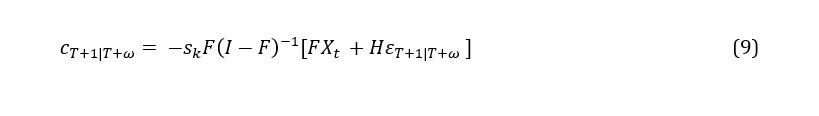
The nowcasting structure implies finding an estimate for  within the quarter having only partial information about the  Hence, this is the case of calculating conditional expectations as data are sequentially released intra-quarter using the Waggoner and Zha (1999) approach. Using equations (5) and (6), we can define the Beveridge-Nelson cycle component at T+1 as follows:

According to Berger et al (2023), this estimated measure of the output gap is not characterized as a high frequency measure, but rather describes how much the flow of the production is below or above the potential. Given the fact that throughout the quarter monthly indicators are released, the nowcast for the output gap can be updated taking into consideration new data set, equivalent to calculating .

Let  be a fraction of the time interval in which all the data corresponding to a reference quarter become available. Thus, following Berger et al (2023), the nowcast for the output gap is

Data set and Results

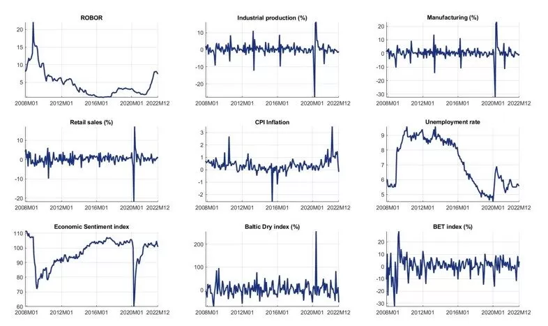
To perform this analysis, we use a data set consisting of nine monthly data series representative of the cyclical position of the Romanian economy to which adds the quarterly real GDP growth. The motivation for the choice of these indicators is that they cover the real economy, financial market, commodity market and confidence indicators, important areas to assess the degree of slack of the economy. The data series cover the sample period of October 2007 to December 2022 and include the global financial crisis and the pandemic. Thus, we use the monthly growth of industrial production, as well as the manufacturing index, retail sales, monthly headline inflation (calculated from the Consumer Price Index) and unemployment rate, which are available on the National Institute of Statistics’ releases. The level of the 3-month ROBOR interest rate is collected from the National Bank of Romania, monthly growth of the Baltic Dry Index is calculated using data from Bloomberg database, the BET index is available on Bucharest Stock Exchange platform and Directorate General produces the Economic Sentiment Indicator for Economic and Financial Affairs (DG ECFIN). The evolutions of the time series are plotted in Fig 1.

The time interval covers both tranquil periods and volatile periods marked by a multitude of shocks, respectively. After the global financial crisis, which produced significant disturbances in the real economy, investors’ confidence and in the financial market, the picture started to outline a relative stability in the dynamics of the indicators. However, this low-volatility period lasted until the beginning of 2020, when the unprecedented COVID-19 pandemic significantly depressed economic activity. We assisted to a drop in industrial production, retail sales, and manufacturing sector along with a decrease in economic sentiment. Due to the authorities’ supporting schemes, the unemployment rate has maintained to levels lower than during the global financial crisis. After that, 2021 was the year of a gradual easing of the restrictions, and in consequence of a strong rebound, which caused bottlenecks in global supply value chains. Moreover, after the recovery of economic activity and demand recovery, inflation has surged to very high levels in many economies, including Romania.

Fig 1. The evolution of data series in the period October 2007 – December 2022

Source: Eurostat, National Institute of Statistics, National Bank of Romania, Bloomberg, author’s calculations

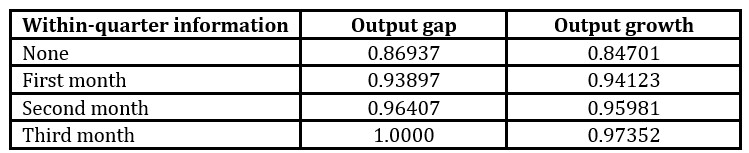
Table 1 presents the correlation coefficients between within-quarter nowcasts and the final estimate for the output gap and output growth. At the beginning of the quarter, having no information from monthly data, the correlation coefficient is higher than 80 %. The indicator increases as new data related to the reference quarter become available.

Table 1. Correlation of nowcasts with output gap and output growth

Source: author’s calculations

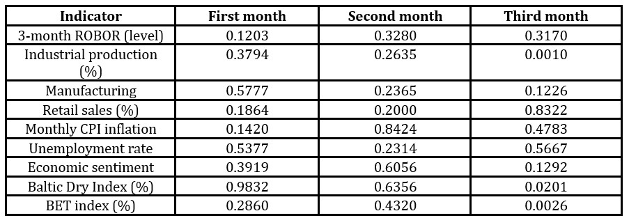
To compare the changes in predictive accuracy for data release in each month of the quarter, we compute the Diebold and Mariano (1995) test, whose p-values are reported in Table 2. According to this, the variables appear to have relatively little impact in improving the nowcast for the output gap. However, a few indicators may improve the reliability of the nowcast in the last month of the quarter, such as industrial production, Baltic Dry and BET indices, all being significant at a 5 % level.  The result of an apparent noninformative CPI inflation for nowcasting the output gap through a multivariate trend-cycle decomposition is close to Berger et al (2023). According to it, this result does not exclude the relationship between the output gap and inflation consistent with the Philips curve.

Table 2. Diebold – Mariano test (p-values)

Source: author’s calculations

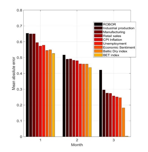
Even though there is little evidence related to the improvements of the final estimate for the output gap, the mean absolute errors between the within-quarter nowcast and the final estimate of the output gap is reduced by almost a half, as in Fig 2. The exception is given by the 3-month interest rate ROBOR whose apparent lack of information is notable. One possible explanation may be the lagged transmission mechanism of the interbank interest rate, a characteristic that was not taken into consideration in this estimation approach. However, the interval accommodates two recessions having different characteristics. On the one hand, the global financial crisis was driven by the downturn in the housing market and spread through linkages in the global financial system, therefore the financial indicators play a crucial role in assessing the degree of inflation pressure in the economy. On the other hand, the nature of the shocks from the unconventional pandemic crisis that hit the world at the beginning of 2020 was completely different. They originate on both the demand side and the supply side, hampering firms’ productive capacity and consumers’ willingness to purchase goods. Thus, it was difficult to identify them, especially when the nature of shocks has been blurred by the authorities’ measures as a response to the pandemic.

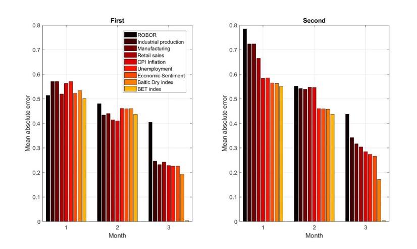
In Fig 3, we display the mean absolute errors after splitting the data set in two equal parts. Given the heightened uncertainty related to the evolution of the COVID-19 pandemic, and the economic events that followed after that (e.g., supply bottlenecks, energy crisis, war in Ukraine), the average percentage point deviation from the final estimate is higher in the second half of the interval than in the first one. Hence, having little information about the economy at the beginning of the quarter, the forecast errors are higher than 0,6 percentage points. Nevertheless, as we expected, the pattern of the decreasing indicator is maintained.

Fig 2. Average percentage point deviation from the final estimate

Source: author’s calculations

Fig 3. Average percentage point deviation from the final estimate in the first and

second halves of the period

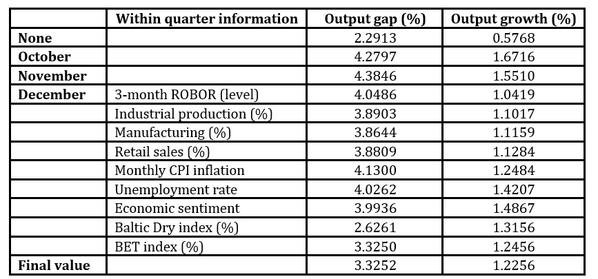
Source: author’s calculationsIn Table 3, we display the within-quarter estimates for Q4 2022 for the output gap and the output growth. We track the evolution of the indicators from the beginning of the quarter, when given no real-time information, the output gap is assessed at around 2,3%. Afterward, in the first two months of the quarter, the favorable dynamics of the indicators (especially economic sentiment and industrial production) appear to increase the level of excess demand in the economy to 4,4%. After the data releases from December, the indicator corrected with real activity indicators dynamics, confidence and financial indicators to a final estimate of around 3,3%. However, the inflation rate still produces the inflationary pressures, given the fact that new data release increases the estimate for both output gap and output growth. Ex-post, it should be noted that according to the release of the provisional data 1 from the National Institute of Statistics on March 8^th, the GDP in Q4 2022 was, in real terms, by 1% higher than the previous quarter.

Table 3. Nowcast for the output gap and the output growth within the last quarter of 2022

Source: author’s calculations

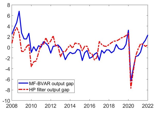
Fig 4. The evolution of the output gap (multivariate BN decomposition versus HP filter)

Source: author’s calculations

For robustness check, we display the historical evolution of the output gap through the multivariate Beveridge-Nelson decomposition relative to the output gap estimated from a simple Hodrick-Prescott (HP) filter, which is the widely used method to decompose real GDP into trend and cycle components. The measure described in this paper is highly correlated with the benchmark HP filter, with a coefficient of 0.63. However, for a better validation of the accuracy of the method, it might be useful to use other advanced filtering techniques that incorporate linkages between variables such as Kalman filter, but this aspect remains for further research.

Conclusions

Given multiple adverse shocks that hit economies from all over the world in recent periods and substantially increased uncertainty, we make an empirical exercise to estimate the Romanian output gap in real time. The Romanian real GDP was recently subject to data revisions that hinder the assessment of this indicator by using conventional filtering techniques. Therefore, this method is reliable for the scope of this analysis and captures the characteristics of the economy. Specifically, after the stability path that followed the global financial crisis, the output gap entered in negative territory immediately after the burst of the pandemic and returned later to its positive values associated with inflationary pressures and an excess of demand. After recovery from the adverse effects of the pandemic shock, given that all monthly variables are available, the estimated value for the output gap in the last quarter of 2022 is around 3%. Hence, the indicator continues to indicate signals for an overheating economy and persistent inflationary pressures.

References

• Alichi, A. (2015), ‘A New Methodology for Estimating the Output Gap in the United States’, IMF Working Paper, 144.
• Alichi, A., Bizimana, O. Laxton, D. Tanyeri, K., Wang, H., Yao, Jiaxiong and Zhang, F. (2017), ‘Multivariate Filter Estimation of Potential Output for the United States’, IMF Working Paper, 106.
• Benes, J., Clinton, K., Garcia-Saltos, R., Johnson, M, Laxton, D., Manchev, P. and Matheson, T. (2010), ‘Estimating Potential Output with a Multivariate Filter’, IMF Working Paper, 285.
• Berger, T., Morley, J. and Wong B. (2023), ‘Nowcasting the output gap’, Journal of Econometrics, 232 (1), 18-34.
• Beveridge, S. and Nelson, C.R. (1981), ‘A New Approach to Decomposition of Economic Time Series into Permanent and Transitory Components with particular attention to the Measurement of the Business Cycle’, Journal of Monetary Economics, 7, 151-174.
• Blagrave, P. Garcia-Saltos, R., Laxton, D. and Zhang, F. (2015), ‘A Simple Multivariate Filter for Estimating Potential Output’, IMF Working Paper, 79.
• Burlon, L. and D’Imperio P. (2020), ‘Reliable real-time estimates of the euro-area output gap’, Journal of Macroeconomics, 64, 2020.
• Diebold, F.X. and Mariano, R.S. (1995), ‘Comparing predictive accuracy’, Journal of Business and Economic Statistics, 13(3), 253-263.
• Harvey, A.C. (1989), Forecasting, Structural Time Series Models and the Kalman Filter, Cambridge University Press.
• Hodrick, R. and Prescott, E. (1997), ‘Post-war Business Cycles: An empirical Investigation’, Journal of Money, Credit and Banking, 29(1), 1-16.
• Juillard, M, Kamenik, O, Kumhof, M and Laxton, D. (2006), ‘Measures of Potential Output from an Estimated DSGE Model of the United States’, CNB Working Paper Series, 11.
• Laxton, D. and Tetlow, R. (1992), ‘A Simple Multivariate Filter for the Measurement of Potential Output’, Bank of Canada, Technical Report, 59.
• Morley, J. and B. Wong (2020), ‘Estimating and Accounting for the Output Gap with Large Bayesian Vector Autoregressions’, Journal of Applied Econometrics, 35 (1), 1-18.
• Morley, J., Palenzuela, D. R., Sun, Y. and Wong, B. (2022), ‘Estimating the Euro Area output gap using multivariate information and addressing the COVID-19 pandemic’, European Central Bank, Working Paper, 2716.
• Orphanides, A. and van Norde, S. (2002), ‘The Unreliability of Output-Gap Estimates in Real Time’, The Review of Economics and Statistics, 84(4), 569-583.
• Primiceri, G. and Justiniano, A. (2009), ‘Potential and Natural Output’, Society for Economic Dynamics.
• Radovan, J. (2020), Estimating Potential Output and the Output Gap in Slovenia Using an Unobserved Components Model. Bank of Slovenia Working Papers, 1.
• Tóth, M. (2021), ‘A multivariate unobserved components model to estimate potential output in the euro area: a production function based approach’, ECB Working Paper Series, No. 2523.
• Veltov, I, Hlédik, T., Jonsson, M. Kucsera, H. and Pisani, M. (2011), ‘Potential Output in DSGE Models’, ECB Working Paper Series, 1351.
• Wallis (1986), ‘Forecasting with an econometric model: The ‘ragged edge’ problem’, Journal of Forecasting, 5(1), 1-13.
• Woodford, M. and Walsh C.E. (2006), ‘Interest and Prices: Foundations of a Theory of Monetary Policy’, Cambridge University Press.